Application of Clustering and Biclustering Techniques to Yeast Metabolic Cycle
<p>Clustering is probably the most used techniques in the analysis of gene expression data. The goal of this technique is to find clusters of genes that have similar expression patterns. The basic assumption behind clustering approaches is that two genes with similar expression patterns are mechanically related. There are many ways in which two genes could be related (when activated by the same transcription factor, when one acts as a transcription factor for the other, when involved in the same biological process and therefore similarly regulated by the cell, etc.). This work will refer to a previously presented research paper -Yeast Metabolic Cycle – which studies genes that have similar expression patterns, we will use them to demonstrate how data mining techniques are applied to bioinformatics. A variety of tools is leveraged in order to apply Clustering and Bi clustering techniques and gains a better understanding of the biological problems we encounter in the field of systems biology.</p>
Introduction
Clustering is a commonly used technique in the analysis of gene expression data. Its goal is to find clusters of genes that have similar expression patterns. The basic assumption behind clustering approaches is that two genes with similar expression patterns are mechanically related. There are many ways in which two genes could be related (when activated by the same transcription factor, when one acts as a transcription factor for the other, when involved in the same biological process and therefore similarly regulated by the cell, etc.). Gene expression analysis alone is generally not sufficient to reveal what kind of relationship links the genes. A cluster analysis consists of three main steps: • The selection of a mathematical representation that reflects the biological issue.
- The identification of an algorithm that solves the mathematical problem by optimizing the score that describes the quality of a cluster or grouping.
- Analysis of results using additional knowledge and data. Choosing a measure of similarity is only a part of the first step. By looking at the clustering algorithms developed in recent years, we can clearly observe the tendency to include more and more biological considerations in the formulation of problems. Groups with a more traditional focus, such as k-means and hierarchical groupings, place each gene exactly in a cluster. Methods of this type are the most widely used and have proven to be useful in many studies.
Bioinformatics & Proteomics Open Access Journal
As a general rule, the assumption that all genes behave similarly under all conditions is too restrictive. To account for this, Biclustering approaches carry out clustering in both dimensions simultaneously: genes and conditions. This allows to find subgroups of genes that exhibit the same response under a subset of conditions, e.g. if a cellular process is only active under these conditions. In addition, if a gene participates in multiple pathways that are differentially regulated, it would be expected for this gene to be included in more than one group, this cannot be achieved by traditional clustering. Several Biclustering algorithms have been proposed in the literature, the strengths and weaknesses of these algorithms are manifested when applied to different biological scenarios. Therefore, it would be worthwhile to test the different approaches and choose which algorithm offers the best results. In this work a data mining study will be carried out using Clustering and Biclustering techniques. HCE3, Expander, BicAT and BicOverlapper tools have been used for the visual analysis of gene expression experiments. In addition to these tools, approaches employing clustering methods have been introduced to systems to classify genes from microarray through multi-agent systems [1, 2] and to obtain genes that show different levels of expression in patients with the same type of cancer [3]. They focus on the integration of expression, relationships and function in order to gain a better understanding of biological problems in the scope of systems biology. This article is structured as follows. Section 2 introduces the experiment. Section 3 details the clustering algorithms and the results obtained. Section 4 describes the applied Biclustering algorithms and the results obtained from their application. The last section shows the obtained conclusions and suggestions for possible future work.
Material and Methods
As in any Data Mining work, the structure consists of the following sections:
- Definition of the problem. The problem is clearly defined and ways of using the data are considered in order to obtain an answer to the problem. These tasks are translated into questions such as the following: o What do we want to find? What types of relationships are we looking for? o Do we want to make predictions from the mining model or just look for interesting associations and patterns? o What result or attribute do we want to predict?
- Preparation of the data. The data that has been identified in the previous step is consolidated and cleaned. Data can be scattered and stored in different formats; it may also contain inconsistencies such as missing or incorrect entries.
- Exploration of data. Data is explored in order to understand the problem, during this process we explore whether the dataset contains faulty data and then devise a strategy to correct the problems or get a deeper description of the behaviours that are typical of the type of problem.
- Generation of the model. The columns of data that will be used in the model are defined, in this way a mining structure is created. The data mining structure is linked to the data source, but does not actually contain any data until it is processed.
- Exploration and validation of the model. Before deploying a model in a production environment, it is advisable to test if it works properly. Normally, when generating a model, several models with different configurations are first created and tested in order to see which one delivers the best results to the problem and to the data.
- Implementation and updating of the model. Once data mining models are in the production environment, depending on the needs different tasks can be performed.
Introduction to the Dataset
The selected dataset is GDS2267: Metabolic cycle: time course of the GSE3431 series (https://www.ncbi.nlm.nih.gov/sites/GDSbrowser?acc =GDS2267). The summary of the dataset is provided: Analysis of nutrient-limited continuous-culture cells at 12-25 minute intervals for 3 cycles. Cells grown under such conditions exhibit robust, periodic cycles in the form of respiratory bursts. Results provide insight into molecular mechanisms responsible for controlling metabolic oscillations.
Preparation of the Dataset
Once the data set is downloaded, we will have to prepare the set to be able to work with it, this will be done by eliminating information that is not relevant to the experiment such as the title, research institute, description, cycles, subsets and discarding control probes and probes without notation. In order to make identification easier, reference numbers will be substituted by the name of each gene, and the GSM by its corresponding T period.
Clustering
HCE3
Clustering algorithms will be applied in this first part of the experiment using the HCE3 tool [3].
Bioinformatics & Proteomics Open Access Journal
Algoritmo HCA One of the features of good clustering algorithms is the ability to determine the number of natural groups in the data set. However, most of the existing clustering algorithms require users to specify the number of groups they want to generate. This requirement causes clustering algorithms to create unnecessary merges or splits, which produce unnatural clusters. On the other hand, the natural number of clusters depends mainly on user preferences or the application itself. A possible solution to this problem is to use the Hierarchical Agglomeration Aggregation (HCA) algorithm that allows the user to control the parameters and determine the appropriate number of groups. Unlike most clustering algorithms, HCA generates a hierarchical structure of groups rather than sets of groups. The HCA algorithm works as follows, if we want to group n data elements, and we have n * (n-1) / 2 similarity (or distance) between the values of all possible pairs of n data elements:
- Initially, each data element occupies a cluster by itself. So there are n groups at the beginning.
- Find a cluster pair whose similarity value is the highest, and make the pair a new cluster.
- Update the similarity values between the new cluster and the remaining groups.
- Steps 2 and 3 apply n - 1 times before there is only one cluster of size n..
There are many possible options for updating the similarity values in the third step. Among them, the most common are linkage-complete, link-media and simple-linkage. Full-binding sets the similarity values between the new cluster and the remaining groups to be the least similar between each member of the new cluster and the rest. The average-linkage uses the average similarity value as new similarity values. We can observe the results of applying the HCA algorithm, represented as dendrograms in Figure 1.
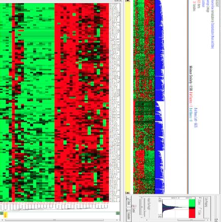
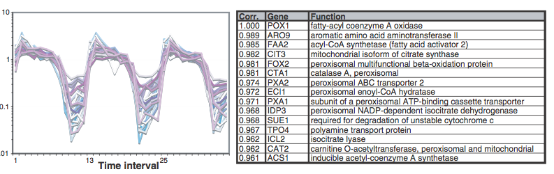
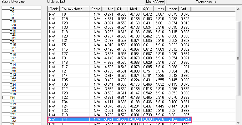
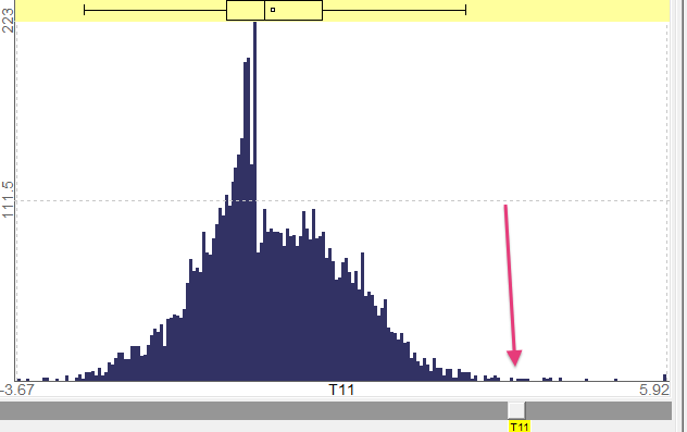
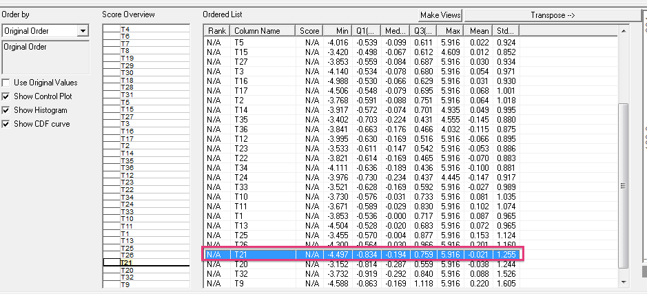
level to POX1, in this way we will be able to see a pattern of similar behaviour between clusters [5, 6]. One of the clusters generated by the HCA algorithm presents in some intervals similar values of the group show in Figure 2. Some of these time intervals may be 11 and 21. In Figure 3 we see the values and the graph of the values of interval 11.
Bioinformatics & Proteomics Open Access Journal
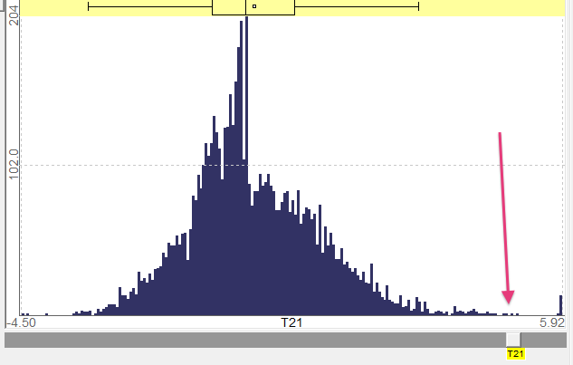
In Figure 5 we observe interval 21, the values are low as in the research work used for reference in this paper.
Bioinformatics & Proteomics Open Access Journal
In Figure 6 we see interval 21, as in the previous image and as it comes in the expression level of the research cluster, has a low level.
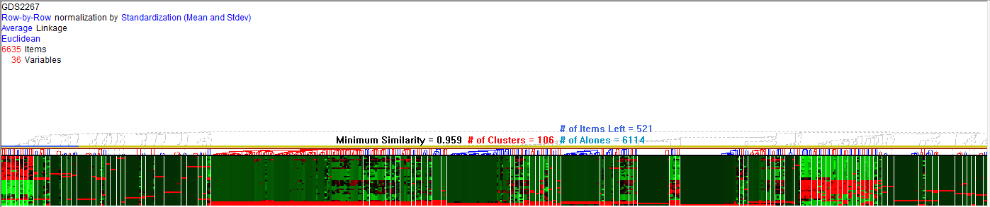
algorithm with a correlation value of 0.959 was applied, obtaining groups with reference genes of 0.961 as indicated in the research paper (Figure 7).
Expander
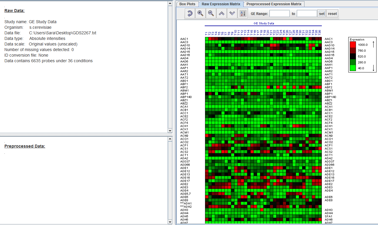
The Expander tool allows you to carry out all the necessary steps in any analysis; Pre-processing of data, normalization, identification of differential genes, application of clustering algorithms and biclustering [7, 8, 9]. Expander is a tool that allows working with the chosen dataset very visually, as shown in Figure 8.
Bioinformatics & Proteomics Open Access Journal
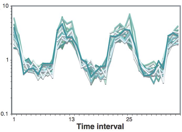
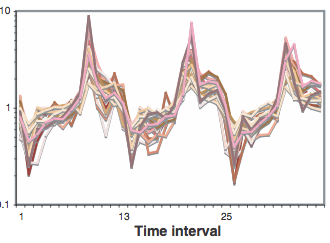
As shown in Figure 9 & Figure 10, the level of expression is first high, then it lowers significantly, then it peaks and drops two times more and finally ends with another high level of expression.
Bioinformatics & Proteomics Open Access Journal
As we see in Figure 11, in intervals 6 and 7 a greater expression occurs, which is repeated in interval 18 and from interval 27 to interval 30.
different values. According to the values of the data set the highest levels of expression occur earlier than those visualized in the research.
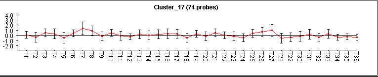
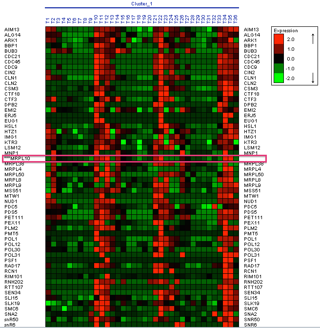
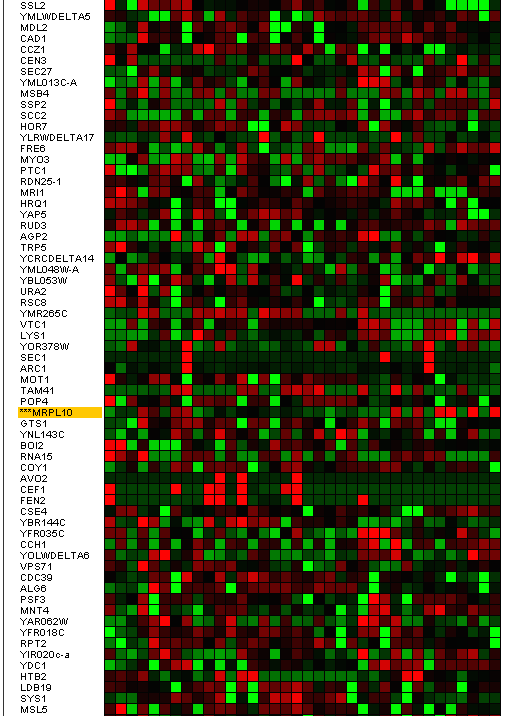
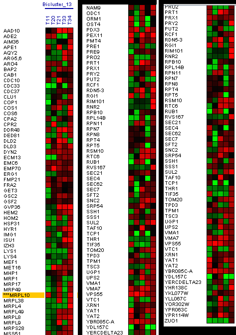
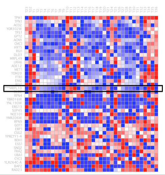
identify clusters of very similar elements (kernels), which probably belong to the same true cluster. The use of this algorithm has generated 27 algorithms; some of these clusters have shown a similar result to the eleventh illustration, MRPL10 gene, (Figure 14).
Bioinformatics & Proteomics Open Access Journal
This cluster has 74 genes with a level of homogeneity of 0.430 and the matrix of expression that it shows, is the one that we can observe in Figure 15.
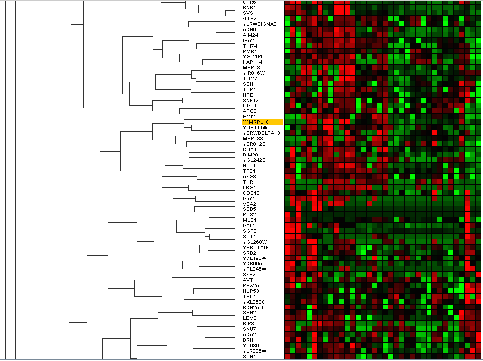
We will then try to cluster with the HCA algorithm, we will perform simple, middle and complete hierarchical clusters. Full-binding sets the similarity values between the new cluster and the remaining groups to obtain the least similarity between each member of the new cluster and the rest. The average-linkage uses the average similarity value as new similarity values. The simple linkage takes it to the maximum, (Figure 16).
Bioinformatics & Proteomics Open Access Journal
consumption that is when it reaches its highest levels of expression. It differs from the previous one in that the distance between two groups is given by the distance between its most distant members. This method is also known as the "farthest neighbour" (Figure 17).
Bioinformatics & Proteomics Open Access Journal
In theory, due to the constitution of this type of cluster we should not find any gene that shares a large number of characteristics and no gene appears as expected.
Biclustering
The common characteristics of clustering techniques are summarized in the search for disjoint sets of genes, such that those genes found in the same cluster present a similar behaviour before all microarray conditions. In addition, each of the genes must belong to a single cluster (and not to none) at the end of the process. Biclustering techniques are presented as a more flexible alternative, since they allow clusters to form not only on a dimensional basis, but also to form biclusters containing genes that exhibit similar behaviour before a subset of microarray conditions. This feature is very important, since it increases the ability to extract information from the same microarray, certain conditions before which a group of genes is not co expressing can be ignored. In the same way, it is also possible to do biclustering in the reverse direction that is, selecting characteristics in terms of a particular subset of genes, although this view has been less studied since it is less biologically interesting. Another important aspect that differentiates biclustering techniques from clustering techniques is the way in which clusters are made, since they can now overlap (several genes can be contained in several biclusters at the same time), there are also genes (or conditions) that have not been included in any subset. This feature gives more flexibility to this type of technique, since it does not oblige to include each gene in a given grouping, instead if a gene’s expression values do not fit any of the patterns, this gene will not belong to any biclusters. Also, it is possible for the same gene to belong to several biclusters, the same gene can participate in several cellular functions simultaneously if in each of the biclusters it is considered a subset of all the experimental conditions. Normally, the problem of locating biclusters in a microarray is more complex than clustering, since there are many more possibilities when grouping the data. The different biclusters obtained can be classified according to different types, which will vary depending on the particular method that is being used to obtain them.
The four main types are listed below:
- Biclusters with constant values. This type of biclusters corresponds to sub matrices that contain identical values in all positions. In them, all genes have the same expression value against all contemplated conditions.
- Biclusters with constant values in rows or columns.
They are biclusters whose genes exhibit a similar behaviour against the conditions, albeit with different expression values for each gene, in the first case. In the case of biclusters with constant values in columns, we collect a set of conditions, where in each of them the genes present the same expression value, but varying from one condition to another. In the second case, the genes exhibit identical behaviour between them.
- Biclusters with consistent values. This type of biclusters gathers relations between genes and conditions that do not have to be direct, but are obtained from a numerical analysis of the data contained in the matrix.
- Biclusters with consistent evolutions. The biclusters that present coherent evolutions present a main difference with respect to the previous ones, since they ignore the concrete numerical values to work with the evolutions or behaviour of the data, seen as symbols.
Expander
The Expander tool also allows you to use biclustering algorithms. Algoritmo Samba: Samba is a novel biclustering algorithm for identifying gene modules that exhibit similar behaviour under a subset of examined biological conditions. Samba is an efficient way to discover statistically significant biclusters in large-scale biological data sets, consisting of hundreds or thousands of diverse experiments. It extends the standard clustering approach by detecting subtle similarities between genes across subsets of measurement conditions and allowing genes to participate in several biclusters. It is therefore more suitable for the analysis of heterogeneous datasets. Following the MRPL10 gene as a reference, 31 biclusters have been made, in three of these biclusters the MRPL10 gene appears. In Figure 18, you can see the first bicluster that has been generated.
Bioinformatics & Proteomics Open Access Journal
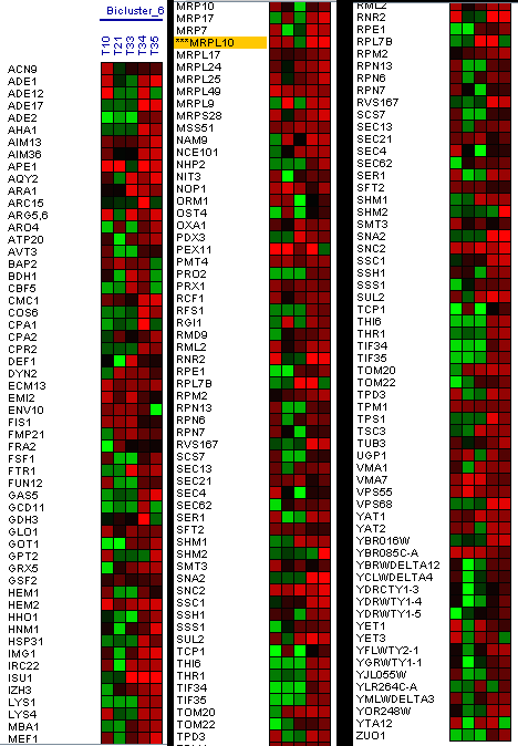
Figure 18: Bicluster with the MRPL10 gene. In the first biclusters we have found genes that appear in the research as the RML2 gene, but we did not obtain a large group of genes similar in expression levels at the same time intervals. The second bicluster does not show genes that would coincide in the phases of oxidation of genes in the same time interval, genes that coincide in these phases in the research that we use as reference (Figure 19).
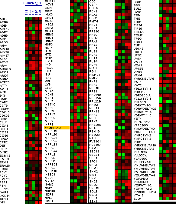
In the last bicluster, the RML2 gene has been found again, but no other gene had been expressed at the same times (Figure 20).
BicOverlapper
The BicOverlapper [10, 12] tool first displays the data on a parallel coordinate axis, representing the expression profiles in lines whose height is proportional to the expression level in each condition (vertical axis). In the background, box diagrams are shown with the distribution of values for each condition. In Figure 21, once a profile is selected we can see the representation of an expression level.
Bioinformatics & Proteomics Open Access Journal
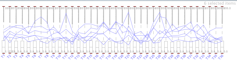
high expression. The heat map is only displayed when a profile is selected, a reduced number of elements.
For the execution of the Bimax algorithm the exact size of the expected biclusters is established, that is to say, the minimum number of genes of each bicluster since otherwise we could finish prematurely, recovering only a small part of the expected biclusters. The parameters that have been chosen for the execution of the algorithm were a minimum of 15 genes per bicluster, and a maximum of 20 groups. After the execution no post - filtering has been performed (Figure 23).
Bioinformatics & Proteomics Open Access Journal
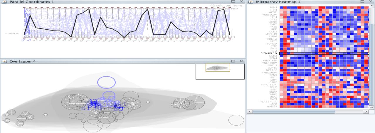
Once executed, several very close clusters have been selected; they are the ones that appear in purple. Among these groups is the MRPL10 gene, let’s see whether the rest of genes in these groups share a similar level of expression (Figure 24).
lower or higher level. An attempt was made to remove this last bicluster group. You can observe the result of deleting this group from the selected clusters in Figure 25.
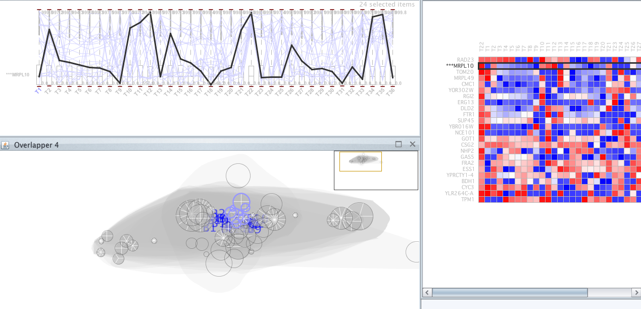
Bioinformatics & Proteomics Open Access Journal
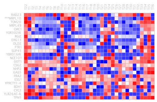
We can also observe that from the middle to the bottom a block is expressed in almost all intervals at lower or higher level. It was attempted to remove this last bicluster group. Figure 26 shows the complete heat map.
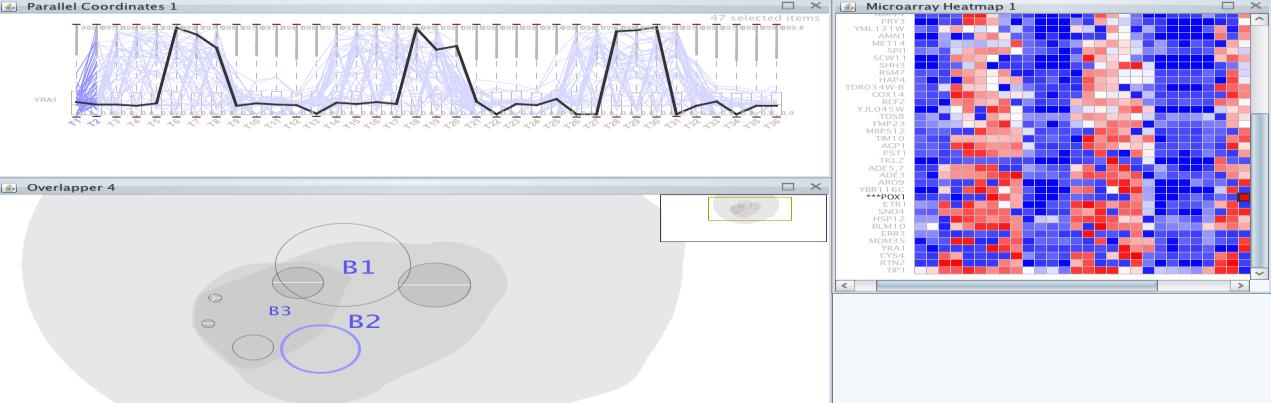
where the background refers to any element of the array that is not a member of any bicluster. The Plaid algorithm conforms to this model by iteratively updating each model parameter to minimize the MSE between the modelled data and the true data. A row release coefficient of 0.8 and a column of 0.2 has been determined and a filtered post is not performed once executed (Figure 27).
Bioinformatics & Proteomics Open Access Journal
A row release coefficient of 0.8 and a column of 0.2 have been determined and post-filtering is not performed once executed. In the selected group we obtained the following set of genes (Figure 28).
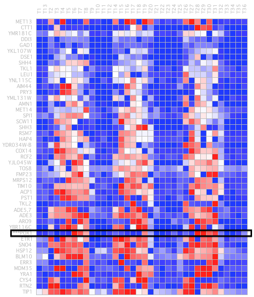
In this set of genes, we find the POX1 gene. This sentinel gene encodes a peroxisomal fatty-acyl coenzyme A (CoA) oxidase. The peak POX1 gene expression occurs as dissolution of the oxygen that has been accumulated during the YMC. In research wherePOX1 was used as a guide, a group of genes was identified with very similar temporal expression patterns, most of which are annotated in coding proteins involved in fatty acid oxidation and peroxisomal function. The coordinated expression of these genes strongly suggests that fatty acid oxidation preferably occurs when the cells fail to breathe. In our bicluster, we have only found another gene called ARO9that appears in the research along with POX1 (Figure 29).
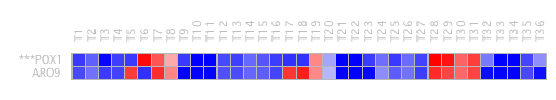
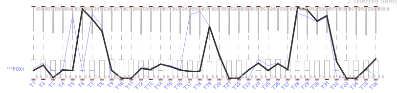
Figure 29: Similar genes in the bicluster generated by Plaid. We see that it has the same expression level at T8, T19 and in the range of T28-T31. The results are equal to those shown in figure 4, both at the expression level and in the non-expression state. There is an average overlap between both genes, as shown in the following illustration. The gene in bold is POX1 and the other gene is ARO9 (Figure 30).
Conclusion
The main objectives of the application of data mining techniques are to predict and group data that present a high degree of similarity. In this work, we focused on the field of bioinformatics, specifically in relation to the raised hypothesis; the recognition of genes that present similar levels of expression. One of the most important techniques is Clustering; its aim is to form groups of genes that share common characteristics. The application of these techniques allows understanding the functionality of genes, their regulation and cellular processes. One of the disadvantages of using this technique is that each cluster of genes is defined using the experimental conditions of the hypothesis. However, the use of Biclustering techniques allows to perform the grouping in two dimensions simultaneously, ie, each gene is selected using only a subset of conditions and only a subgroup of genes is Bioinformatics & Proteomics Open Access Journal
chosen from each condition of a bicluster. Giving the identification of genes and subgroups with similar conditions applying Clustering on the rows and columns at the same time. These techniques are ideal when there are clusters of genes in a dataset that share common characteristics that are unknown a priori. The degree of agreement of the results of the study based on yeast research, such as Saccharomyces cerevisiae, with reality depends to a great degree on the quality and reliability of the data used for the study. Some of the data on genes seemed to have been duplicated, and with different values in the data set leaving us with the first occurrence of the repeated genes and deleting the repetitions, this fact may have been able to alter the results of the results. In nature, most of the behaviours of living things are governed by some kind of reason or pattern, this is why data mining has many diverse applications. Thus, the field of data mining is being researched profusely and continues to experience great developments, not only in commercial applications but also in academic work.
Conflict of Interests
Relevant Genes in Expression Analysis between Young and Older Women with Triple Negative Breast Cancer. J Integr Bioinform 12(4): 278.
4. Santamaría R, Therón R, Quintales L (2008)
BicOverlapper: a tool for bicluster visualization. Bioinformatics 24(9): 1212-1213.
5. Castellanos-Garzón JA, Ramos J, González-Briones
A, de Paz JF (2016) A Clustering-Based Method for Gene Selection to Classify Tissue Samples in Lung Cancer. In 10th International Conference on Practical Applications of Computational Biology & Bioinformatics, Springer, Cham pp: 99-107.
6. González-Briones A, Ramos J, De Paz JF, Corchado
JM (2017) An Agent-Based Clustering Approach for Gene Selection in Gene Expression Microarray. Interdisciplinary Sciences: Computational Life Sciences 9(1): 1-13.
7. Santamaría R, Therón R, Quintales L (2014)
BicOverlapper 2.0: visual analysis for gene expression. Bioinformatics 30(12): 1785-1786.
8. Seo J, Shneiderman B (2004) A rank-by-feature framework for unsupervised multidimensional data exploration using low dimensional projections. IEEE Symposium on Information Visualization pp: 65-72.
The author declares that there is no conflict of interests regarding the publication of this paper.
Acknowledgment
The research of Alfonso González-Briones has been co-financed by the European Social Fund (Operational Programme 2014-2020 for Castilla y León, EDU/310/2015 BOCYL).
References
-
Sharan R, Maron-Katz A, Shamir R (2003) CLICK and EXPANDER: a system for clustering and visualizing gene expression data. Bioinformatics 19(14): 1787-1799.
-
Tu BP, Kudlicki A, Rowicka M, McKnight SL (2005) Logic of the yeast metabolic cycle: temporal compartmentalization of cellular processes. Science 310(5751): 1152-1158. et al. (2010) Expander: from expression microarrays to networks and functions. Nature protocols 5(2): 303-322.
-
González-Briones A, Ramos J, De Paz JF, Corchado JM (2015) Multi-agent System for Obtaining
-
Seo J, Shneiderman B (2005) A rank-by-feature framework for interactive exploration of multidimensional data. Information visualization 4(2): 96-113.
-
Seo J, Bakay M, Chen YW, Hilmer S, Shneiderman B (2004) Interactively optimizing signal-to-noise ratios in expression profiling: project-specific algorithm selection and detection p-value weighting in Affymetrix microarrays. Bioinformatics 20(16): 2534-2544.
-
Shamir R, Maron-Katz A, Tanay A, Linhart C, Steinfeld I, et al. (2005) EXPANDER–an integrative program suite for microarray data analysis. BMC bioinformatics 6(1): 232.
-
Ulitsky I, Maron-Katz A, Shavit S, Sagir D, Linhart C,
- Carbon Code for Analysis of Protein Stability in Protein Mutation
- Number of Contiguous Amino Acids in Nanon of 16A Diameter
- Identification of Hub Genes and Pathways in Cervical Cancer by Statistical and Bioinformatics Analysis
- Effect of Dietary Inclusion Levels of Moringa Olerifera Oil on the Growth Performance and Nutrient Retention of Broiler Starter Chicks
- Proteomics Loans in Kinetoplastids during the Last Decade
- “Identification of SARS-CoV-2 in Human Genome based on Protein Dynamics Conversion and Target Genes Marking via Bioinformatics Approaches”