Empirical Model of the Functioning of Aquatic Ecosystems

Introduction

Aquatic ecosystems can be formed in the range of environmental variables only that has been well demonstrated in the Sládeček model [1] (Figure 1). On the base of the trophic pyramid in aquatic ecosystems are placed the primary producers like an algae and cyanobacteria. The relationships between algal biodiversity and environmental conditions are determined by adaptation level of the species and the community as a whole. Bio indication is based on the principal of congruence between community composition and complexity of environmental factors [2]. However, it is still a problem to define the role of particular environmental variables as well as to predict the community’s response to environmental change. The governments, scientists, managers, and the public are interested in assessing the health of ecosystems [3]. Therefore, the problem of assessment of the ecosystem state and predicting of its development still important up to now in purpose of understood how we could to assess the risk factors and to manage it [4]. The first step in this way is to collect information about methods and examples of its application. How we can recognize the structure of algal community change. Across the investigation of the species richness in community and cell abundance. It can give us the material for structural Index Shannon calculation. On the base of same data, we can calculate Index of Saprobity the value of which can be inserted into the Sládeček ecosystem model. If the community changes its structure, the index Saprobity S have the amplitude of its value [2]. Structural index Shannon fluctuated also. Important, that we calculate both indices on the base of same data for entire community. Therefore, we can to compare how one index changes over other. Monitoring of biological elements is a key aspect of the assessment of the chemical and ecological status within the framework of the Water Framework Directive. The all existing biological methods for assessing water quality definition of biological conditions in aquatic objects were summarizes in [5]. The next step is the development of the predictive models as an instrument for assessment of the state of aquatic ecosystems and it was a number [6, 7, 8, 9, 10]. Ecological modelling has a long story from hierarchical [11, 12, 13, 14, 15] to structurally dynamic (SDMs) [16, 17, 18, 19] models. So, the ‘ODD’ (Overview, Design concepts, and Details) protocol was created in purpose to standardize the published descriptions of individual-based and agent-based models. During the last years are developed models with using GIS and neural networks and Self-Organizing Maps [20, 21, 22]. In purpose of our model is interesting to include some information variable such entropy in the models and empirical data to the model [23, 24, 25, 26]. We assume that the structure of the aquatic community, expressed by the Shannon diversity index, as well as species richness, has a definite relationship with the indicators of the trophic status of the water body, expressed by indices of organic pollution according to Sládeček and Watanabe. In any case, the existed models can work for the some community of some natural or experimental object. The aim of our work was to collect known information about entire aquatic ecosystems from freshwater habitats and to summarize it in three variables (Species richness, Index Shannon, and Index Saprobity) relationships.

Results and Discussion

The microalgae community is ideal for this purpose because the microalgae cell size corresponds to each species body shape and usually fast varied in the bright range during vegetation season. Therefore, the species- specific individual mass and species richness are varied under environmental factors change very fast. The main cells dimensions can be different not only in different water bodies but also in the time series samples in water body the same. As a result, we can explore increasing of the total cell surface with increasing of cell number and decreasing cell volume when algae bloom in the aquatic object. The total cell surface is positively correlated with the intensity of metabolic processes in the autotrophic organisms [27, 28]. This is most clearly expressed when blue-green algae bloom. Diatoms, on the contrary, are the most conservative group of organisms in relation of its dimensions, and the distribution of cell size over latitude. However, they are represented basically the same tendency as the other group of organisms and show a negative correlation with latitude [29]. That is, in the south of the equator in the size of the cells is greater than in the north where cell size decreased with increasing latitude under stressful conditions. Thus, to reduce the size of microalgae cells lead not only well-known eutrophication, expressed in bloom, but climatic stress also [30]. Therefore, if we know the environmental factors such as salinity stress that lead to a decrease in cell volume (increase in cell surface for metabolic rate), and species richness of algae we can assume about its influence on the intensity of primary production processes [31]. The main property of the Sládeček’s model is the water quality over the all possible variables from distilled water to technical solution. In the model on Figure 1 is marked by blue the variables in which can exist entire aquatic ecosystems with primary producers at the base. The related environmental variables are consist only one first quadrant and related each other in the range of the Water Quality Classes (I-V at the Figure 1) [1]. Index Saprobity S is also included in the model and ranged from 0 to 4. Nevertheless, self-purification in aquatic ecosystems is follow in the direction of yellow arrow in the second quadrant also where normal trophic pyramid cannot develop but the bacteria and Heterotrophs are present. Our worked area was the first quadrant.

Click to enlarge

Figure 1: Saprobity model based on [1]. Each quadrant (Katarobity, Limnosaprobity, Eusaprobity, and Transsaprobity) symbolize four main groups of variables with respect to purity and pollution (Sládeček, [1]). The symbols: x, o, β, α, p, denote the self-purification zones, which, in turn, are used to determine Classes of water quality (I-V, [2]). The blue quadrants correspond to the freshwater ecosystems. Yellow arrow gives the self- purification process direction.

The work with algal communities is always included calculation of Species richness, Index of Saprobity S, and Index Shannon especially for the phytoplankton community. On the base of our large more than thirty years’ experience, we take our data about algal communities’ species richness and abundance from aquatic communities of diverse water bodies of Eurasia. Our database are included twelve years monthly research in the Artyomovskoye, Pionerskoye, Bogatinskoye reservoirs and rivers from the Russian Far East, as well as study in 1992-1995 in the Velikoe Lake (Vladimirskaya district of Russia). We studied the Teletzkoye Lake in the Altay Natural Reserve, Moscow district small lakes and reservoirs, the Onega Lake, Kola Peninsula small lakes, the small lakes in the Kostyanoy Nos Natural Reserve (Russian Arctic). We studied algal communities from the Tadjik Depression rivers and lakes, from the Georgian rivers and lakes, especially on the protected areas and Natural Reserves. Large rivers of Ukraine such as Southern Bug and Dnieper give us data about its phytoplankton. Ukrainian estuaries Kuyalnik and Sasyk on the Black Sea coast were also studied in its phytoplankton. Data included also seasonally studied algal communities from nine rivers and its tributaries as well as from forty-two small aquatic habitats of Israel. The Pakistan Rivers Swat and Kabul give us also data about algal communities. Indian small lakes in Kolkata district were included also. Our study of the Songhua River in China gives the algal communities data. We also have some data from the personal communication of Prof. Tamara Mikheeva about the Berezina and Svisloch rivers (Belarus) algal communities. Taken data included species richness, Index Shannon, Index saprobity S and for some communities also Watanabe organic pollution index. We include in our model also data from the papers of Toshiharu Watanabe and its colleagues about lentic and riverine communities of Japan. Whereas the Index Saprobity S and environmental variables data can be correlated across the Sládeček’s model and classification ranks, the Index Shannon and species richness data including is represent some difficulties [2]. Figure 2 show long-term fluctuation of these parameters for the Artyomovsk Reservoir in Far East. Can be seen, species richness decreased (a) together with much fluctuated Shannon index H (b) that slightly clear in the yearly values (c). Therefore, we cannot recognize correlation low between these three variables on the sample of one aquatic object ecosystem because the succession process takes so long time.

Click to enlarge

Figure 2: Long-term fluctuation of algal species richness (a), Shannon index H (b) and year-averaged Shannon index H in the Artyomovsk Reservoir, Russian Far East. The dashed lines are the power trend line, the straight line in (a) is the linear trend line. In this reason, we are take the formation about these three variables from our more than 30 years’ experience as well as collected data from more than 2,500 communities from published papers and books, and from our unpublished data and personal communication. The first who compare the saprobity indices DAIpo with species richness and index Shannon was T. Watanabe with his lab [32, 33]. His data of species richness in diatom communities and index Shannon are distributed over his DAIpo index of saprobity. We compare DAIpo with the Sládeček’s index of saprobity S ranges and correlate both in one system [34, 35]. Therefore, all data about environmental variables and Indices of Saprobity S range from the Sládeček’smodel can be correlate with the data of DAIpo, species richness, and Index Shannon from the Watanabe’s data. More of them, we include in the water quality Classes range all our investigated data for three parameters. As a result, the distribution of environmental variables ranges can be correlated not only with the Sládeček’s indices S but also with the Watanabe DAIpo indices and therefore with the Index Shannon data from his papers. On the first step of our modelling, we take data about the Shannon index from all our investigation as well as from the Watanabe’s data for streaming and standing water communities and compare it with the Saprobity S and DAIpo values [36, 37]. Figure 3 show the distribution of Shannon index H over the DAIpo. Can be seen, Index Shannon in studied communities is fluctuated between 0 and 5 with the sharp border from the upper part of distribution field and more dissolved from the bottom. We do not include all shared data about H in purpose to see how the different communities can be represented on the field of H. In the full picture, the field of H distribution is black as a whole. In Figure 3 can be seen that more abundant streaming communities’ data are fills up all field of H, whereas the standing water bodies communities’ data are fluctuated in the narrow range and fills up only part of the figure. In any case, the symmetrical distribution of the community structure indicator Index H can be recognized. That means that the community change its structure over the environmental variables trend [2] in the full amplitude of the ecosystem parameters. Can be mentioned, in the Watanabe system DAIpo is lower in the polluted waters and up to 100 in natural clear waters whereas in the Sládeček system the pollution increased with indices from 0 to 4. The part of the H-field on the Figure 3 the DAIpo amplitude from 40 to 100 is reflect the communities from the natural clean or with full self-purification processes in ecosystem. Range of DAIpo 30-40 can be marked as Dangerous for community. Community with DAIpo in 20-30 range is under risk and 15-20 in critical stage. If the community have 0-15 DAIpo, its state developed very fast and the ecosystem can collapsed.

Click to enlarge

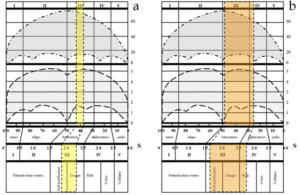
Figure 3: The distribution of Shannon index H over the Index DAIpo. The same distribution was constructed for the species richness in algal and cyanobacteria community over DAIpo. We combined together the scale of the DAIpo, the Sládeček Index S scale, the water quality classes and the fields formed by the Shannon index H and the number of species in the community. Figure 4 show the results of combining. The important thing in the figure is the scale of the Water Quality Classes that correspond to amplitudes of chemical and biological variables in the classification system [2]. The self-purification zones from Sládeček’s model (Figure 1) are correlated also with the Water Quality Classes. Sládeček’s zones are placed in the Figure 3 and correlate with the ecosystem state periods that we marked on the Shannon index H distribution base. Now we can see only one-two parameters in the ecosystem for assess of its state. So, Figure 5 show change of the Index S value amplitude in the Qishon River ecosystem from 2003 to 2005 when pollution and ecosystem disturbance were sharply increased [38]. Can be seen, in 2003 index S was correspond to narrow interval in Class III, whereas in 2005 index S was increased in its range in Class III and Class IV and correspond to the ecosystem risk state. Many other samples of ecosystem dynamic were revealed in our experience [39, 40, 41].

Click to enlarge

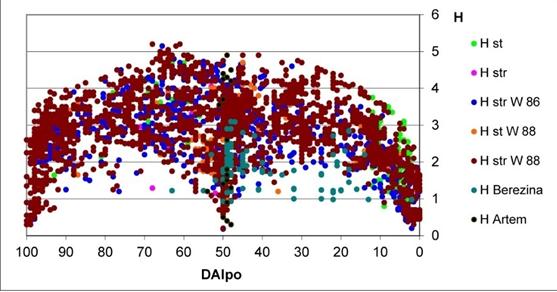
Figure 4: The empirical model of the aquatic ecosystem state on the base of algal community data distribution of Shannon index H and Species richness over the Index DAIpo, Index S, and Water Quality Classes. Species richness in our model shows some different distribution. At the top of Figure 4, it can be seen that in the cleanest xenosaprobic and oligotrophic waters, the number of species is minimal. In mesotrophic and eutrophic waters, the number of species is greatest with a maximum between these categories. In the process of further increasing the trophic load and, correspondingly, an increase in the index S, the number of species in the community gradually decreases, and in highly contaminated hypertrophic waters it again reaches a minimum. By the way, dotes in the Figure 3 that corresponds to the Artyomovsk reservoir are placed in the middle part of the figure H and have high amplitude of fluctuation, high species richness in communities and narrow amplitude of index S fluctuation. The ecosystem state can be assessed as in the border of natural clean waters and full self-purification. It is important for monitoring and makes decision system because his reservoir is one of the major drinking water sources for Primorsky district in the Russian Far East.

Click to enlarge

are as follows. Encyonema minuta as one of the permanent components of pioneer succession stages is characterized by a progressive increase in the association of cells, the growth of colonies along with the growth of biomass. Somewhat later, Didymosphenia geminata and other species with similar saprobity develop a variety of algal community. The appearance of Tabellaria characterizes the climax stage, in which the diversity of algae reaches about fifty species (Figure 4, top); most of them have a narrow ecological niche. The introduction of Aulacoseira species into the Tabellaria complex occurs near the inflection of the community biodiversity curve and, apparently, marks the passage of the climax succession stage. Reduction of biological diversity (the descending part of the right half of the H field) occurs in the reverse order in relation to the above tendencies of progressive development and is characterized, first of all, by the loss of Tabellaria by the removal of the climax stage. Domination turns to species with a broad ecological tolerance. The structure of the colonies develops regressively along the path of dissociation and a decrease in cell size. In the final stages of the regressive series, coloniality degrades to individual, single cells.

The general pattern is a reduction in the size of the cells of each species population, with a simultaneous increase in total biomass and a reduction in the number of species. Biomass, as a community response to a change in the trophic base, is also linked by diversity through saprobity indices. In the left part of the figure, biomass increases due to the increase in the number of species, and in the right part due to the growth of the population. Morphology, more precisely the dimensional gradient of the species, is also reflected in the model. On the left are larger cells of the population. With succession progress to the right, the cells decrease in size with an increase in the trophic base, increasing the surface, but still within the limits of each species variability. To interpret the obtained results, it is of decisive importance that, with a unidirectional increase in the level of impact, reversibility of the development of biological diversity is observed at the first stages of progressive development of algal community. Then, after the crisis phase - a fracture of the empirical curve - in the succession stage of regressive development there is a decrease in the indices of diversity with a continuing increase in trophic load. In Figure 4 can be seen that the ascending and descending branches are symmetrical, and reversibility is manifested in different, distinctly pronounced tendencies at the morphological and biocenosis levels. The upward part of the figure (the left part of figure 4) in our interpretation is due to the fact that at the initial stages of anthropogenic influence the trophic base expands, which leads to the stabilization of the habitat of algal communities. Diversity is increases due to narrowly specialized species with simultaneous growth of association such as coloniality and morphological complication. These tendencies culminate near the fracture of the biological diversity field near the highest values of the Shannon index H and species richness, which corresponds to the moment in the evolution of the ecosystem, when the further increase in the impact and trophic base has a destabilizing effect by removing dependence on the trophic resource. The emergence of Aulacoseira near the inflection of the biodiversity curve means that, due to the excessiveness of trophic resources, the effectiveness of their use ceases to be a factor of competitiveness, when ineffective species that are capable of rapid population growth are put forward. The development of this trend (the right-hand side of Figure 4) leads to a simplification of the community structure and a decrease in the level of biological diversity, which, starting at a certain point, is accompanied by a sharp drop in biological productivity and threatens the complete destruction of the ecosystem, up to single finds of high-pollution indicator species, such as Gonium pectorale. Discussion of the regularities in which the community changes leads individual authors to the conclusion that the structure of communities after reaching the climax stage or removing it as a result of the impact can change in two ways: continuing the growth of diversity or lowering the diversity along the same curve but in the opposite direction. The assumption of such a branching of the succession opportunities of the community is called bifurcation. Considering empirical data and changing natural communities, we have to recognize that bifurcation is not observed in natural algal communities of algae. Perhaps, for a double direction of development of communities, the symmetry of structures is accepted in the "natural" and "anthropogenic" stages of succession. On our model, it can be seen that the right and left wing of the figure have similar outlines. Thus, development does not go in the opposite direction, but in the progressive direction - on the model, the transition from the left wing to the right. The empirical dependence of the change in the biodiversity of algal communities in the process of growth of the trophicity of the water body revealed by us seems to be applied to communities of other trophic levels of the ecosystem. In the work of K.D. Carlander, a picture is given that reflects the relationship between the production indicators of ichthyocenoses and their species diversity [42]. His figure shows that the cloud of points forms a figure similar to the one we constructed, but with a slightly compressed right wing. The points are located more rarely, apparently in connection with the logarithmic scale of the abscissa axis, but their field (not outlined by the author) leaves no doubt about the similarity of the contours. From the distribution shown, K.D. Carlander does not make an empirical conclusion but mathematically determines the approximate linear trend line direction of changes in species diversity. It should also be noted that attempts to draw the resulting curves and/or trend lines for such a scatter of points do not give a positive result, the lines are almost parallel to the abscissa axis, and this is a dead-end path. Thus, it can be assumed that the regularity revealed by us applies to both the higher and the lower levels of the ecosystem. Since the biotic part of the ecosystem is built according to the law of the trophic pyramid it can be concluded that our model is applicable for assessing the state of the aquatic ecosystem as a whole [2].

Conclusion

On the base of our large experience and available references, we constructed empirical model that combine together the data about species richness, indices saprobity S and DAIpo with information Shannon index of more than 2,500 algal and cyanobacteria communities from diverse water bodies of Eurasia. The fields of the data points in coordinates of Index Saprobity and Index Shannon, and Index Saprobity and Species richness in the model can be described as the major succession trends with the trophic base increasing. We correlate the scales of both mentioned saprobity indices in purpose to enrich the model by the environmental data from the V. Sládeček model [1], water quality classification [2] and the diversity data from the recent papers of T. Watanabe [32, 33, 36, 37]. Remarkable that our model is based not only on the experience data and can be therefore empirical, but also the model reflects major successional stages in algal communities. We define the community parameters that reflect natural undisturbed community, self-purified ecosystem range of variables as well as critical parameters up to variables in which the ecosystem can collapsed. The main successional stages in the model coincided with the self-purification zones in the Sládeček model [1]. Whereas known up to now models are worked with the data limited to a particular water body and, therefore they can predict the development of only this system and only for a short period of time, our model can be used as a prognostic instrument for the large period for any aquatic ecosystem. Moreover, we would never have been able to observe the passage of all stages of the succession process in water bodies from zero trophicity to the maximum possible in polluted waters, since the duration of our life is incommensurable with the duration of the succession process in ecosystems. We recognize only part of the succession process when try to predict its direction in the certain waterbody. Thus, our empirical model makes it possible to work on assessing the state of any possible within the parameters of the first quadrant of the Sládeček model of an aquatic ecosystem and predict its development. The model can be used not only for the ecosystem state assessment but also for predicting of given ecosystem development in the succession way. Therefore, if we know current position of studied ecosystem, we can include its parameters for the decision making in respect of the aquatic object diversity protection or even restoration. The model also provides us with parameters for assessing reversible or irreversible changes in the ecosystem of the water body that very important to know for protection or restoration of given object.

Acknowledgements

The work was partly supported by the Israeli Ministry of Absorption.