Statistical Investigation of B-fields in Cores and Filaments using JCMT/SCUPOL Legacy Survey Archival Data
SCUPOL, the polarimeter for SCUBA on the James Clerk Maxwell Telescope was used for polarization observations of 104 regions at 850 μm wavelength and 15” resolution in the mapping mode by Matthews BC, et al. [1]. They presented the polarization values and magnetic field morphologies in these regions. In this work, we took the opportunity to use this big legacy survey data to investigate further the collective statistical properties of the measured polarization in different starforming regions containing cores and filaments. We did not reproduce the polarization maps but used the polarization value catalogs to investigate the statistics of distributions. In some of these regions, the data from Combined Array for Research in Millimeter-wave Astronomy (CARMA) polarization observation at 1.3 mm wavelength and 2.”5 resolution was also available from the TADPOL survey. We used that data and compared it with JCMT/SCUPOL values. We also study how the direction of outflows appears to relate the mean B-field direction from large scale (JCMT observation at 15”) to small scale (CARMA observation 2.5”) for the nine core regions common in both.
Abbreviations
CARMA: Combined Array for Research in Millimeter-wave Astronomy; RAT: Radiative Alignment Torque; KDE: Kernal Density Estimation; AGB: Asymptotic Giant Branch; BG: Bok Globules, SC/PC: Starless or Prestellar Cores; SFR: Star- Forming Regions; YSO: Young Stellar Objects; VeLLOs: Very Low Luminosity Objects.
Introduction
Magnetic fields are crucial components in the star formation process, significantly influencing the dynamics involved [1, 2, 3, 4, 5, 6]. The study of magnetic field morphology within the interstellar medium has been extensively advanced through observations of polarization caused by the alignment of interstellar dust grains. This phenomenon was initially discovered by Hall JS [7], and Hiltner WA [8, 9]. For many years, the prevailing theory was that paramagnetic relaxation was responsible for aligning these rapidly rotating dust grains with the magnetic field. However, this alignment mechanism has faced significant challenges, both observationally and theoretically, revealing numerous limitations in its explanatory power [10, 11].
The ’Radiative Alignment Torque’ (RAT) theory is currently the most widely accepted mechanism for the alignment of interstellar dust grains. Initially proposed by Dolginov Z, et al. [12] and later fully developed by Draine T, et al. [13] and Lazarian A, et al. [11], this theory posits that in the presence of anisotropic radiation, the transfer of torques from photons to paramagnetic and non-spherical or elongated dust grains induces a rapid spin-up of these grains. As a result of this rotation, the grains acquire a net magnetic moment through the Barnett effect, causing them to precess around the magnetic field. This magnetic moment further drives the angular momentum of the grains to precess around the magnetic field in a manner known as Larmor precession, ultimately aligning the grains’ angular momentum parallel to the magnetic field lines. Over the past decade, numerous predictions of this theory have been substantiated, though the finer details of the mechanism and its components remain areas for further investigation [14].
When dust grains aligned by the interstellar magnetic field absorb radiation at shorter wavelengths, they re- emit this energy at longer wavelengths, specifically in the far infrared, millimeter, or sub-millimeter regions of the spectrum. The emitted radiation is polarized along the grains’ long axis, meaning the electric field vector of the polarized emission is perpendicular to the plane-of-sky component of the local magnetic field.
Magnetic fields are typically well-ordered across large spatial scales, ranging from approximately 100 parsecs to 1 parsec [15]. However, on smaller, subparsec scales, magnetic fields can exhibit random orientations. This disarray is attributed to processes such as ambipolar diffusion and turbulent magnetic reconnection diffusion, which disrupt the coherence of the magnetic field lines [16, 17, 18, 19, 20, 21].
In the paper, we used the JCMT/SCUPOL data from legacy surveys in some cores and filaments and the TADPOL archival data in some regions which are common in both studies. We used the available polarization measurements to infer: mean B-field orientations, the statistical distribution of polarization values, relations between large (JCMT at 15” resolution) and small (CARMA at 2.5” resolution) scale B-fields, and the relation between outflow orientations with mean B-field orientations at different spatial scales. This work uses the opportunity to do statistical analysis of the available polarization measurements which was not presented in the original paper of JCMT/SCUPOL legacy survey [1]. Here section 2 presents data acquisition details, section 3 shows the results of our analysis, and section 4 summarises this study.
Methodology
The JCMT-SCUPOL data
In this study, we utilized SCUPOL data to explore the statistical properties of magnetic fields within core and filamentary structures. This dataset, derived from the comprehensive work The Legacy of SCUPOL: 850 µm Imaging Polarimetry from 1997 to 2005, encompasses polarimetric observations performed by SCUPOL, the polarimeter for SCUBA on the James Clerk Maxwell Telescope (JCMT), covering the period from 1997 to July 2005 [1]. While SCUBA facilitated simultaneous observations at both 850 µm and 450 µm, the 450 µm data were either unavailable or had insufficient sensitivity for the regions analyzed. As a result, our study is exclusively based on 850 µm observations, targeting various astrophysical environments, including cores, filaments, ridges, galaxies, planetary nebulae, asymptotic giant branch (AGB) stars, and supernova remnants, with a particular emphasis on cores and filaments. Within core regions, we focused on four primary categories: Bok globules (BG), starless or prestellar cores (SC/PC), star- forming regions (SFR), and young stellar objects (YSO). Data reduction and processing were accomplished using the Starlink software suite, including the SURF, KAPPA, POLPACK, and CURSA packages, yielding an angular resolution of 15” and the detailed data reduction procedure is described in Matthews BC, et al. [1]. Further, we supplemented our analysis with data from additional specific cores of interest.
The CARMA Data
To examine the dynamic interplay between outflows from core regions and magnetic fields across different spatial scales, we incorporated data from the TADPOL survey, as detailed in the publication TADPOL: A 1.3 mm Survey of Dust Polarization in Star-Forming Cores and Regions [2]. This survey presents 1.3 mm polarimetric observations from the Combined Array for Research in Millimeter-wave Astronomy (CARMA), encompassing dust polarization data for 30 star- forming cores and 8 star-forming regions. The TADPOL data provide high-resolution magnetic field maps on a more localized scale, with a spatial resolution of 2.5”, offering a finer level of detail than the JCMT/SCUPOL observations, thereby enhancing our ability to probe magnetic field structure on smaller scales. The data reduction methodology for the CARMA observations is thoroughly described in Hull CLH, et al. [2].
Results
Statistical Analysis of the Core Polarization Data
Magnetic Fields in the Cores: To examine the morphology of magnetic fields within core regions, we selected a subset of 45 cores from the dataset presented by Matthews BC, et al. [1], which involved dust polarization observations conducted at a wavelength of 850 µm using the JCMT/SCUPOL system, achieving a resolution of 15”. In this study, data were sampled at an angular resolution of 10” with select regions binned to 20”, as elaborated in Matthews BC, et al. [1] and included only areas exhibiting significant polarization vectors. The selected regions meet the stringent criteria of p/dp > 2, dp < 4%, and I
> 0, where I represents the Stokes intensity parameter and p denotes the polarization degree.
To investigate the variation in outflow direction in relation to the mean magnetic field direction across different scales, we further narrowed our focus to nine core regions shared between the 30 star-forming cores and 8 star-forming regions observed in the Combined Array for Research in Millimeter-wave Astronomy (CARMA) at a wavelength of 1.3 mm with a resolution of 2.5” [2]. These nine core regions are common to both the CARMA and JCMT observations, allowing for a comparative analysis of magnetic field dynamics in these astrophysical environments.
Histogram of θB and Scatter Plot of p vs. θB: In the JCMT/ SCUPOL dataset, the position angles (θE) of the polarization E-vector at a wavelength of 850 µm are provided. To derive the position angle (θB) of the B-vector, θE is rotated by 90°, after which a histogram is constructed to illustrate the distribution of θB for each individual core region. The blue dotted line in these histograms represents the mean position angle of the magnetic fields (θBmean) across the respective core regions.
Additionally, the scatter plot depicting the degree of polarization (p) against the B-vector position angle (θB) reveals the relationship between polarization and magnetic field orientation. Figure 1 displays the histogram of θB alongside the scatter plot of p versus θB for selected cores. The error bars in the scatter plots indicate the uncertainties associated with each p and θB measurement.
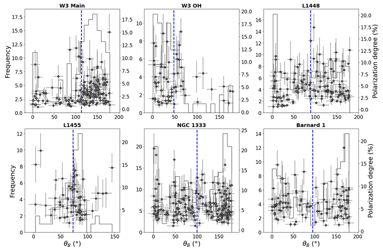
Figure 1: Histogram of θB and scatter plot of polarization degree (p) vs. θB with error bars for the core regions. The histograms illustrate the distribution of magnetic field vector position angles (θB), with a blue dotted line in each plot indicating the mean position angle (θBmean) for the respective core regions. The scatter plots depict the polarization degree (p) across various position angles in these regions, with error bars representing the uncertainties associated with each value of p and θB. The scatter plots, inclusive of error bars, reveal that the majority of data points cluster within the ranges of 113
- < θB < 175
- and 0.8% < p < 6% for the W3 Main region, as well as within 0° < θB < 75° and 1% < p < 16% for the W3 OH region. In contrast, the remaining plots exhibit a greater dispersion in both p and θB values, indicating a more complex relationship in those regions.
Histogram and Kernal Density Estimation (KDE) of the difference between θminor and θBmean: The angle (θminor) formed by the minor axis of an ellipse, which is roughly fitted to the core region, with respect to the vertical line (the north-south direction) is measured in an anticlockwise manner. This ellipse is approximated either inside or outside the outermost contour of the core region, as delineated in Matthews BC, et al. [1]. The B-vector position angles (θB) for individual cores are derived by adding 90° to the θE values provided in the SCUPOL dataset. Subsequently, the mean B-vector position angle (θBmean) is computed for each core. Figure 2 illustrates the measurement procedure for θminor, θBmean, and ∆θ with respect to the reference direction (northsouth).
![Figure 2: Measurement of the minor axis angle (θminor), the mean magnetic field angle (θBmean), and the angular difference between these orientations (∆θ) for the W3 Main region. The color map is adapted from Matthews BC, et al. [1], as the polarization map was not re-created in this study.](/fulltextimages/13485/fig_2.png)
| Name | RA (J2000) | DEC (J2000) | Object type | θ (◦) minor | θ (◦) Bmean | ∆θ(◦) | Distance (kpc) |
|---|---|---|---|---|---|---|---|
| W3 Main | 02 25 35.44 | +62 06 16.4 | SFR (HM) | 17 | 113 ± 9 | 96 ± 9 | 1.95 [19] |
| W3 OH | 02 27 03.83 | +61 52 24.8 | SFR (HM) | 141 | 48 ± 9 | 93 ± 9 | 1.95 [19] |
| L1448 | 03 25 38.80 | +30 44 05.4 | YSO (Class 0) | 80 | 89 ± 10 | 9 ± 10 | 0.250 ± 0.050 [20] |
| L1455 | 03 27 41.31 | +30 12 39.4 | SFR (LM) | 45 | 73 ± 9 | 28 ± 9 | 0.250 ± 0.050 [20] |
| NGC 1333 | 03 29 11.11 | +31 13 20.2 | SFR (HM) | 89 | 100 ± 9 | 11 ± 9 | 0.320 [21] |
| Barnard 1 | 03 33 17.88 | +31 09 32.9 | SFR (LM) | 99 | 95 ± 9 | 4 ± 9 | 0.250 ± 0.050 [20] |
| HH211/IC348 | 03 43 56.70 | +32 00 51.9 | SFR (LM) | 120 | 114 ± 6 | 6 ± 6 | 0.250 ± 0.050 [20] |
| L1498 | 04 10 52.60 | +25 10 00.0 | SC/PC | 36 | 123 ± 9 | 87 ± 9 | 0.14 ± 0.02 [22] |
| L1527 | 04 39 53.90 | +26 03 10.0 | YSO (Class 0) | 35 | 75 ± 9 | 40 ± 9 | 0.140 ± 0.010 [23] |
| IRAM 04191+1522 | 04 21 56.91 | +15 29 46.1 | YSO (Class 0) | 164 | 64 ± 8 | 100 ± 8 | 0.140 ± 0.010 [23] |
| L1544 | 05 04 17.23 | +25 10 43.7 | SC/PC | 55 | 61 ± 10 | 6 ± 10 | 0.140 ± 0.010 [23] |
| NGC 2071 IR | 05 47 04.85 | +00 21 47.1 | SFR (HM) | 80 | 89 ± 10 | 9 ± 10 | 0.400 [24] |
| IRAS 05490+2658 | 05 52 13.24 | +26 59 33.3 | SFR (HM) | 77 | 71 ± 10 | 6 ± 10 | 2.1 [25] |
| Mon R2 IRS | 06 07 46.16 | -06 23 22.5 | SFR (HM) | 110 | 51 ± 8 | 59 ± 8 | 0.950 [26] |
| MON IRAS 12 | 06 41 05.81 | +09 34 09.0 | SFR (HM) | 115 | 67 ± 5 | 48 ± 5 | 0.800 [27] |
| CB 54 | 07 04 21.07 | -16 23 20.09 | BG | 70 | 78 ± 10 | 8 ± 10 | 1.1 [28] |
| L183 | 15 54 08.96 | -02 52 43.9 | SC/PC | 80 | 86 ± 9 | 6 ± 9 | 0.15 [29] |
| ρ Oph A | 16 26 26.45 | -24 24 10.9 | SFR (IM) | 96 | 103 ± 8 | 7 ± 8 | 0.139 [30] |
| ρ Oph C | 16 27 00.10 | -24 34 26.7 | SFR (IM) | 25 | 88 ± 9 | 63 ± 9 | 0.139 [30] |
| ρ Oph B2 | 16 27 27.97 | -24 27 06.8 | SFR (IM) | 170 | 93 ± 9 | 77 ± 9 | 0.139 [30] |
| L43 | 16 34 35.57 | -15 47 00.6 | SC/PC | 39 | 101 ± 9 | 62 ± 9 | 0.17 [29] |
| NGC 6334A | 17 20 19.55 | -35 54 42.3 | SFR (HM) | 158 | 97 ± 10 | 61 ± 10 | 1.7 [31] |
| GGD 27 | 18 19 12.00 | -20 47 30.9 | SFR (HM) | 117 | 74 ± 10 | 43 ± 10 | 1.7 [32] |
| CRL 2136 IRS 1 | 18 22 26.48 | -13 30 15.1 | SFR (HM) | 100 | 106 ± 10 | 6 ± 10 | 2 [33] |
| Serpens Main Core | 18 29 49.34 | +01 15 54.6 | SFR (LM) | 65 | 97 ± 8 | 32 ± 8 | 0.310 [34] |
| CL 04/CL 21 | 18 37 19.39 | -07 11 31.8 | SFR (HM) | 108 | 119 ± 9 | 11 ± 9 | 0.770 [35] |
| G28.34+0.06 | 18 42 52.40 | -03 59 53.9 | SFR (HM) | 89 | 104 ± 10 | 15 ± 10 | 4.8 [36] |
| IRAS 18437-0216 | 18 46 23.23 | -02 13 45.4 | SFR (HM) | 84 | 77 ± 9 | 7 ± 9 | 6.6 [37] |
| W48 | 19 01 45.45 | +01 13 04.5 | SFR (HM) | 10 | 76 ± 8 | 66 ± 8 | 3.4 [38] |
| R Cr A | 19 01 53.65 | -36 57 07.5 | SFR (HM) | 99 | 100 ± 10 | 1 ± 10 | 0.130 [39] |
| W49 | 19 10 13.60 | +09 06 17.4 | SFR (HM) | 100 | 100 ± 6 | 0 ± 6 | 11.4 [40] |
| W51 | 19 23 42.00 | +14 30 33.0 | SFR (HM) | 90 | 98 ± 9 | 8 ± 9 | 7.5 [41] |
| IRAS 20081+2720 | 20 10 13.99 | +27 28 36.9 | SFR (LM) | 14 | 29 ± 9 | 15 ± 9 | 0.700 [42] |
| AFGL 2591 IRS | 20 29 24.72 | +40 11 18.9 | SFR (HM) | 150 | 114 ± 9 | 36 ± 9 | 1.5 [43] |
| IRAS 20188+3928 | 20 20 38.75 | +39 38 03.9 | SFR (HM) | 98 | 110 ± 9 | 12 ± 9 | 0.4 – 4 [44] |
| S106 | 20 27 17.32 | +37 22 41.3 | SFR (HM) | 155 | 96 ± 8 | 59 ± 8 | 0.600 [45] |
| G079.3+0.3 | 20 32 23.62 | +40 19 44.0 | SFR (LM) | 117 | 130 ± 9 | 13 ± 9 | 1 [36] |
| S140 | 22 19 18.00 | +63 18 49.0 | SFR (HM) | 92 | 87 ± 8 | 5 ± 8 | 0.900 [46] |
| S146 | 22 49 28.56 | +59 55 08.6 | SFR (HM) | 89 | 89 ± 9 | 0 ± 9 | 5.2 [47] |
| Cepheus A | 22 56 17.80 | +62 01 49.0 | YSO (Class 0/I) | 147 | 71 ± 8 | 76 ± 8 | 0.730 [48] |
| S152 | 22 58 50.14 | +58 45 01.0 | SFR (HM) | 71 | 122 ± 9 | 51 ± 9 | 5 [49] |
| NGC 7538 | 23 13 45.54 | +61 27 35.7 | SFR (HM) | 90 | 113 ± 8 | 23 ± 8 | 2.8 [50] |
| S157 | 23 16 04.00 | +60 02 06.0 | SFR (HM) | 64 | 79 ± 10 | 15 ± 10 | 2.5 [51] |
Table 1: Table for calculating ∆θ (= |θBmean − θminor|).
The analysis summarized in Table 1 reveals a striking alignment in certain cores, notably W49 and S146, where the ∆θ value approaches 0° , defined as ∆θ = θBmean θminor. This close alignment signifies that the mean magnetic field in these cores is precisely oriented along the minor axis. In contrast, this parallelism is less pronounced or absent in other cores.
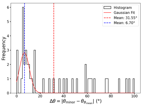
Figure 3: Histogram of the angular difference, ∆θ (θBmean θminor), for the core regions. This histogram illustrates the distribution of ∆θ values computed for the cores identified in Table 1, with a red curve superimposed to depict the Gaussian fit to the data. The vertical dashed lines, colored red and blue, represent the mean value of ∆θ and the peak of the fitted Gaussian curve, respectively, providing insight into the central tendency and most probable value of the angular difference.
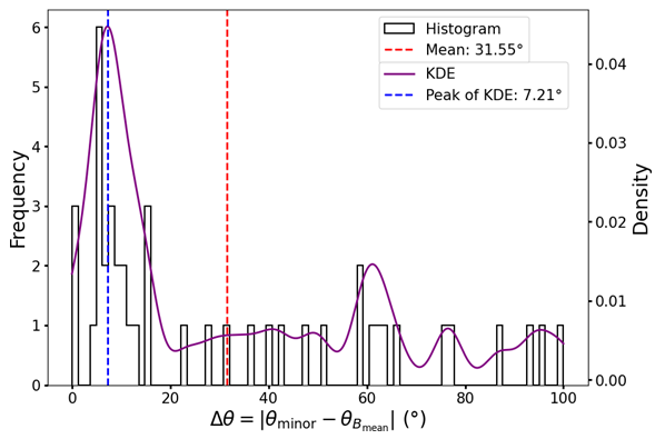
Figure 4: KDE plot (depicted by the purple curve) of the angular difference, ∆θ = (θBmean θminor), for the core regions, overlaid on the histogram of ∆θ values derived from the cores listed in Table 1. The red and blue dashed lines indicate the mean value of ∆θ and the peak of the KDE curve, respectively, highlighting the central tendency and the most probable value of the angular difference within the data distribution.
To illustrate the distribution of ∆θ, we generated a histogram, displayed in Figure 3, with a red curve representing a Gaussian fit. This fit peaks at approximately 6.70°, indicating a prevalent trend in ∆θ alignment. Figure 4 presents the Kernel Density Estimate (KDE) plot of the ∆θ histogram, peaking at around 7.21°, reinforcing the observed alignment trend. Both the Gaussian fit and KDE plot peaks suggest that the majority of cores exhibit a minor axis orientation closely aligned with the mean magnetic field direction.
From Table 1, we calculate the mean ∆θ value as 32° ± 9°. This average supports the notion that the magnetic field direction within these core regions predominantly aligns with the minor axis. Such an orientation is consistent with observations by SCUPOL, highlighting a significant degree of parallelism between the magnetic field and structural morphology within these astrophysical cores. Additionally, Soam A, et al. [52] showed that the mean magnetic field direction with the minor axes of a limited sample of five cores is approximately 37°, further implying that the mean B-field is nearly parallel to the minor axis of these core regions.
The dispersion of ∆θ values within the core regions is approximately 30.19°. This substantial dispersion indicates that the B-field position angles exhibit a random alignment in the JCMT-SCUPOL observations.
Overall, this study provides a statistical representation of the magnetic field morphology in the plane of the sky, consistent with previous hypotheses.
Difference between Outflow and Mean B-field Orientation: In the TADPOL survey, a detailed examination of dust polarization was conducted using observations from the Combined Array for Research in Millimeter-wave Astronomy (CARMA) at a wavelength of 1.3 mm, targeting 30 star-forming cores and 8 star-forming regions. Through these observations, the small-scale magnetic field orientation (χsm) was determined with a resolution of 2′′.5 within the identified core regions. Additionally, the angle of the outflow ejection (χ0) was also calculated [2].
Prior to section 3.1.4, the mean magnetic field position angle (θBmean) for each individual core region was derived from JCMT/SCUPOL data. Notably, θBmean represents the mean value of the B-vector position angle on a large scale, which is significantly larger than the scale of the CARMA observations.
All angles—χsm, χ0, and θBmean —are measured in an anticlockwise direction with respect to the north-south orientation.
Between the CARMA and JCMT surveys, we identified nine common core regions that facilitated a comparative analysis of the variation in outflow direction between large- scale and small-scale magnetic fields, which we visualized using a Kernel Density Estimate (KDE) plot.
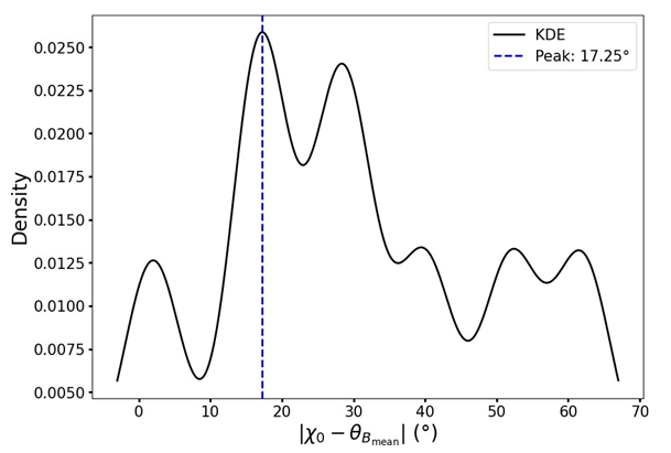
Figure 5: KDE plot depicting the angular difference between θBmean and χ0 for the nine cores observed in both JCMT and CARMA datasets. The blue dashed line marks the peak of the KDE curve for θBmean χ0, which occurs at 17.25◦. This value suggests that, on a large scale, the outflow direction for these cores is nearly aligned with the mean magnetic field orientation.
The KDE plot depicting the angular difference between θBmean and χ0 is shown in Figure 5. In this plot, the blue dashed line highlights a peak value of θBmean χ0 around 17.25°, while the mean value, calculated from Table 2, is approximately 31° 8°. These findings collectively suggest that the outflow emanating from the core regions aligns closely with the mean magnetic field direction on large scales. In a study by Soam A, et al. [52], an examination of five cores containing Very Low Luminosity Objects (VeLLOs) showed that the outflows in three of these cores exhibit a significant tendency to align with the magnetic field orientation within the surrounding envelope.
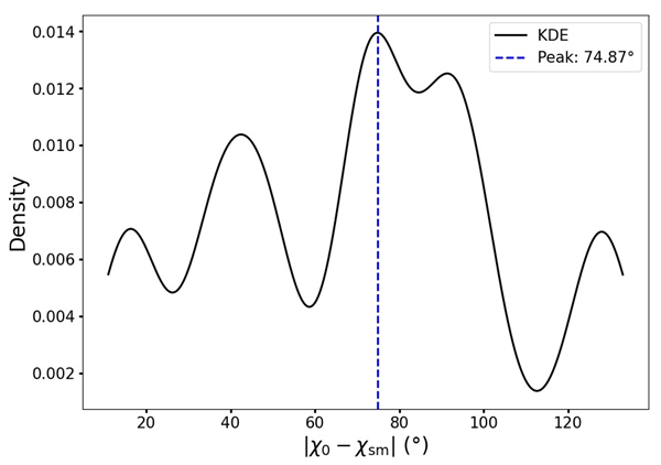
Figure 6: KDE plot depicting the angular difference between χsm and χ0 for the nine cores observed in both JCMT and CARMA datasets. The blue dashed line marks the peak of the KDE curve for χ0 χsm, which occurs at 74.87◦. This value suggests that, on a small scale, the outflow direction for these cores is nearly perpendicular to the mean magnetic field orientation.
Following this, we present the KDE plot for the angular difference between χ0 and χsm in Figure 6. Here, the blue dashed line indicates a peak value of χsm - χ0 at 74.87°, while the mean value, derived from Table 2, is approximately 70° ± 36°. These results imply that, at smaller scales, the outflow direction within the core regions is predominantly orthogonal to the mean magnetic field orientation. This finding is consistent with Hull CLH, et al. [2], who observed that, on smaller scales, the outflow direction tends to be nearly perpendicular to the mean magnetic field position angle.
| No. | Name | p (%) | χ (◦) sm | χ (◦) 0 | θ (◦) Bmean | |θ − χ | (◦) Bmean 0 | |χsm − χ | (◦) 0 |
|---|---|---|---|---|---|---|---|
| 1 | L1448C | 5 ± 2 | 26 ± 37 | 97 | 89 ± 10 | 40 ± 10 | 71 ± 35 |
| L1448N | 5 ± 2 | 112 ± 32 | 161 | 89 ± 10 | 40 ± 10 | 71 ± 35 | |
| 2 | NGC 1333- IRAS 2Ac | 6 ± 2 | 70 ± 23 | 59.5 | 100 ± 9 | 62 ± 9 | 16 ± 25 |
| SVS 13 | 6 ± 2 | 6 ± 24 | ... | 100 ± 9 | 62 ± 9 | 16 ± 25 | |
| NGC 1333- IRAS 4A | 6 ± 2 | 56 ± 20 | 18 | 100 ± 9 | 62 ± 9 | 16 ± 25 | |
| NGC 1333- IRAS 4B | 6 ± 2 | 84 ± 34 | 0 | 100 ± 9 | 62 ± 9 | 16 ± 25 | |
| NGC 1333- IRAS-4B2 | 6 ± 2 | 55 ± 20 | 76 | 100 ± 9 | 62 ± 9 | 16 ± 25 | |
| 3 | HH211MM | 9 ± 2 | 164 ± 32 | 116 | 114 ± 6 | 2 ± 6 | 48 ± 32 |
| 4 | L1527 | 7 ± 2 | 3 ± 8 | 92 | 75 ± 9 | 17 ± 9 | 89 ± 8 |
| 5 | CB 54 | 6 ± 2 | 32 ± 42 | 108 | 78 ± 10 | 30 ± 10 | 76 ± 42 |
| 6 | VLA 1623 | 5 ± 1 | 23 ± 48 | 120 | 103 ± 8 | 17 ± 8 | 97 ± 48 |
| 7 | Ser-emb 8 | 7 ± 2 | 7 ± 44 | 123 | 97 ± 8 | 27 ± 8 | 37 ± 33 |
| Ser-emb 8(N) | 7 ± 2 | 83 ± 15 | 107 | 97 ± 8 | 27 ± 8 | 37 ± 33 | |
| Ser-emb 6 | 7 ± 2 | 172 ± 33 | 135 | 97 ± 8 | 27 ± 8 | 37 ± 33 | |
| 8 | NGC 7538 | 4 ± 1 | 52 ± 62 | ... | 113 ± 8 | ... | ... |
| 9 | CB 244 | 12 ± 3 | 170 ± 49 | 42 | 94 ± 7 | 52 ± 7 | 128 ± 49 |
Table 2 consolidates the computed values of θBmean χ0 and χsm - χ0 across the nine cores examined, providing a clear summary of the observed alignment trends at both large and small scales.
Kernel Density Estimation plot of χsm (CARMA data) and θBmean (JCMT data): This study demonstrated that the alignment between the large-scale and small-scale magnetic fields in core regions was not entirely parallel, as illustrated in Figure 7. The smallscale observations, which provided a magnified view of the larger scales, revealed a more intricate structure of the magnetic field orientation deep within the cores. This observed misalignment between the largescale and small-scale magnetic field directions contributed to a low degree of polarization (p). This phenomenon suggested that the alignment of dust grains was disrupted by the random orientations of magnetic fields at smaller scales [2]. The transition from large to small spatial scales unveiled a significantly more complex polarization pattern, characterized by distorted magnetic field geometries. Furthermore, evidence of hourglass morphologies was apparent in the densest regions of some cores, indicating the intricate interplay between the magnetic fields and the surrounding matter.
![Figure 7: The smallscale observations, which provided a magnified view of the larger scales, revealed a more intricate structure of the magnetic field orientation deep within the cores. This observed misalignment between the largescale and small-scale magnetic field directions contributed to a low degree of polarization (p). This phenomenon suggested that the alignment of dust grains was disrupted by the random orientations of magnetic fields at smaller scales [2]. The transition from large to small spatial scales unveiled a significantly more complex polarization pattern, characterized by distorted magnetic field geometries. Furthermore, evidence of hourglass morphologies was apparent in the densest regions of some cores, indicating the intricate interplay between the magnetic fields and the surrounding matter.](/fulltextimages/13485/fig_7.png)
Statistical analysis of the Filament Polarization Data
In this section, the magnetic field morphology in the filament regions is studied in detail.
Magnetic Field in Filament Regions: In this study, the data were sampled at a resolution of 10”; in certain instances, it was binned to 20”, as detailed in Matthews BC, et al. [1]. The dataset exclusively comprises regions where significant polarization vectors were detected, adhering to the criteria of p/∆p > 2, ∆p < 4%, and I > 0. To investigate the morphology of magnetic fields within filament regions, we selected six filaments that were observed using the JCMT/SCUPOL at a wavelength of 850 µm and a resolution of 15” [1].
Histogram of θB and scatter plot of p vs. θB and KDE plot of the difference between θmajor and θBmean: The histogram illustrating the position angle (θB) of the B-vector, along with the scatter plot depicting the degree of polarization (p) against θB (Figure 8), was constructed following the methodology employed for the core regions. These histograms reveal the distribution of θB, with the blue dotted line indicating the mean value of the magnetic field position angle, denoted as θBmean. The scatter plot presents the degree of polarization at varying angles θB, with error bars representing the uncertainties associated with the corresponding p and θB values.
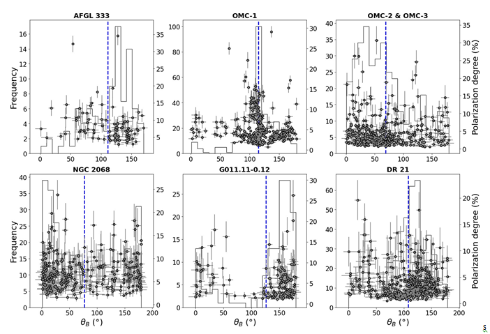
Figure 8: Histogram of θB and scatter plot of p vs. θB with the error bars for the filament regions. The histograms show the distribution of B-vector position angles (θB) and the blue dotted line in each of the histograms shows the mean value of B-vector position angle (θBmean) in those individual filament regions. The scatter plots show the polarization degree (p) at different position angles for those filament regions and the error bars are the uncertainties in each p and θB value.
The scatter plots, inclusive of error bars, demonstrate that the majority of data points are confined within the following ranges: 113° < θB < 160° and 3% < p < 10% for the AFGL 333 region; 90° < θB < 130° and 1% < p < 16% for the OMC-1 region; 0° < θB < 100° and 0.8% < p < 8% for the OMC- 2 & OMC-3 regions; 125° < θB < 177° and 1% < p < 10% for the G011.11-0.12 region; and 75° < θB < 175° and 0.6% < p <
![Figure 9: Measurement of the minor axis angle (θmajor), the mean magnetic field angle (θBmean), and the angular difference between these orientations (∆θ) for AFGL 333 region. The color map is adapted from Matthews BC, et al. [1], as the polarization map was not re-created in this study.](/fulltextimages/13485/fig_9.png)
| Name | RA (J2000) | DEC (J2000) | Object type | θ (◦) major | θ (◦) Bmean | ∆θ(◦) | Distance (kpc) |
|---|---|---|---|---|---|---|---|
| AFGL 333 | 02 28 08.81 | +61 29 25.0 | SFR (HM) | 19 | 111 ± 7 | 92 ± 7 | 1.95 [19] |
| OMC-1 | 05 35 14.5 | -05 22 33.0 | SFR (HM) | 10 | 115 ± 4 | 105 ± 4 | 0.414 ± 0.007 [53] |
| OMC-2 & OMC-3 | 05 35 26.9 | -05 09 58 | SFR (LM) | 166 | 69 ± 7 | 97 ± 7 | 0.414 ± 0.007 [53] |
| NGC 2068 | 05 46 37.64 | +00 00 33.1 | SFR (LM) | 62 | 77 ± 8 | 15 ± 8 | 0.400 [24] |
| G011.11-0.12 | 18 10 33.99 | -19 21 36.9 | SFR (HM) | 55 | 126 ± 8 | 71 ± 8 | 3.6 [36] |
| DR 21 | 20 39 01.50 | +42 19 38.0 | SFR (HM) | 176 | 108 ± 9 | 68 ± 9 | 3 [54] |
Table 3: Table to calculate ∆θ = |θmajor − θBmean| for individual filament region.
The mean value of ∆θ (defined as θBmean θmajor), indicating the deviation of the mean B-field direction from the major axis of the filament, is computed to be 75° 7° as derived from Table 3. This finding suggests that the major axis of the filament is nearly perpendicular to the direction of the mean magnetic field.
This observation is further corroborated by the KDE plot (Figure 10), which illustrates the peak value of the KDE of (∆θ) mean at 70°, indicated by the blue dashed line.
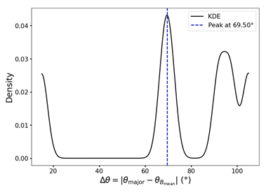
The dispersion of ∆θ values within the filament regions is approximately 29.83°. This substantial dispersion highlights the random alignment of the B-field position angles within these filamentous structures.
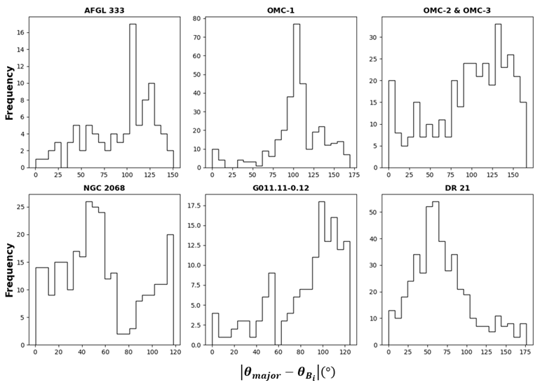
Histogram of the difference between θmajor and θBi: The histogram depicting the difference between θmajor and θBi (Figure 11) elucidates the extent to which the observed position angle of the magnetic field, θBi, deviates from the major axis of each filament region.
For all filament regions analyzed, the observed differences between θmajor and θBi indicate a predominant trend where the major axis of the filament is nearly perpendicular to the corresponding observed position angle of the magnetic field (θBi).
Discussion
Star Formation in Core Region
In the core region, two distinct categories of particles are present: charged particles, such as electrons and ions, and neutral particles, including atoms and molecules. The dynamics of these particles differ fundamentally due to their interactions with the magnetic field. Charged particles are constrained to traverse along the magnetic field lines, following a helical trajectory, while neutral particles, experiencing no magnetic force, possess the freedom to move in any direction.
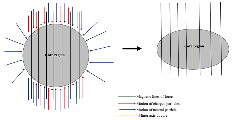
As depicted in Figure 12, both charged and neutral particles enter the core region by aligning with the magnetic field lines. However, only the neutral particles can approach the core from various directions.
This results in a greater degree of contraction along the magnetic field lines, causing the minor axis of the core region to align closely with the direction of the magnetic lines of force [55, 56, 57, 58]. This phenomenon, known as “ambipolar diffusion”, plays a pivotal role in star formation. The extent of contraction along the direction of the magnetic field is contingent upon the degree of ionization; a lower level of ionization leads to a correspondingly diminished contraction.
Through the process of ambipolar diffusion, a core that is initially sub-critical characterized by magnetic energy that surpasses gravitational energy, thus preventing collapse can transition to a super-critical state, where gravitational forces dominate over magnetic influence, allowing for collapse and the potential initiation of star formation. Figure 12 illustrates a cartoon model of ambipolar diffusion, elucidating the alignment of the mean magnetic field direction with the minor axis of the core and demonstrating how the infall of particles within the core region contributes to the onset of star formation.
Star Formation in Filament Region
Filamentary structures typically arise in regions characterized by weaker magnetic fields that are influenced by the surrounding gas flow. Gilberto CG, et al. [59] have demonstrated the U-shaped morphology of the magnetic field in proximity to the filament. In these regions, the gas flows align with the direction of the magnetic field, thereby necessitating that the plane of the sky component of the magnetic field remains perpendicular to the long axis of the filament.
In our investigation, we conducted a comprehensive statistical analysis of the magnetic field morphology within the plane of the sky. Our findings indicate that the orientation of the magnetic field is predominantly parallel to the minor axis of the core region while remaining nearly perpendicular to the major axis of the filament.
Conclusion
- The statistical analysis of the combined polarization measurements in the cores and filaments is summarized as follows:
- The statistical evaluation of the magnetic field morphology within core regions reveals that the plane of the sky component of the mean magnetic field is predominantly parallel to the minor axis of the core regions.
- In several core regions, the outflow direction aligns closely with the large-scale mean magnetic field; however, it exhibits a near perpendicular relationship with the mean magnetic field measured on smaller scales.
- The mean magnetic field direction within core regions demonstrates variability between large and small scales, and this misalignment contributes to a reduction in the degree of polarization (p).
- The analysis of magnetic field morphology in filament regions indicates that the plane of the sky component of the mean magnetic field is largely perpendicular to the major axis of the filament regions.
- In filament regions, the major axis of the filament is almost perpendicular to the observed B-vector position angle values.
Acknowledgements
This research has made use of the SIMBAD database, operated at CDS, Strasbourg, France. We also acknowledge the use of NASA’s SkyView facility (http://skyview.gsfc. nasa. gov) located at NASA Goddard Space Flight Center. We acknowledge the usage of archival data from JCMT/SCUPOL and CARMA/TADPOL surveys.
P.P acknowledges Dr. Archana Soam for her invaluable guidance and insightful suggestions, which greatly enriched this project and contributed significantly to its successful completion. Software: APLpy, Astropy [60, 61, 62].
References
-
Matthews BC, McPhee CA, Fissel LM, Curran RL (2009) The Legacy of SCUPOL: 850 µm Imaging Polarimetry from 1997 to 2005. The Astrophysical Journal Supplement Series 182(1): 143-204.
-
Hull CLH, Plambeck RL, Kwon W, Bower GC, Carpenter JM, et al. (2014) TADPOL: A 1.3 mm Survey of Dust Polarization in Star-forming Cores and Regions 213(1): 13.
-
Liu J, Zhang Q, Qiu K (2022) Magnetic field properties in star formation: A review of their analysis methods and interpretation. Frontiers in Astronomy and Space Sciences 9: 943556.
-
Li HB, Goodman A, Sridharan TK, Houde M, Zhi-Yun Li, et al. (2014) The link between magnetic fields and cloud/ star formation. Protostars and planets, pp: 101-123.
-
Shu FH, Adams FC, Lizano S (1987) Star formation in molecular clouds: observation and theory. 25: 23-81.
-
McKee CF, Zweibel EG, Goodman AA, Heiles C (1993) Magnetic Fields in Star-Forming Regions Theory. In: Levy EH, Lunine JI (Eds.), Protostars and Planets 3: 327.
-
Hall JS (1949) Observations of the Polarized Light from Stars. Science 109(2825): 166-167.
-
Hiltner WA (1949) On the Presence of Polarization in the Continuous Radiation of Stars. SAO/NASA Astrophysics Data System (ADS) 109: 471.
-
Hiltner WA (1949) Polarization of Light from Distant Stars by Interstellar Medium. Science 109(2825): 165.
-
Hough JH, Aitken DK, Whittet DCB, Adamson AJ, Chrysostomou A (2008) Grain alignment in dense interstellar environments: spectropolarimetry of the 4.67-µm CO-ice feature in the field star Elias 16 (Taurus dark cloud). Monthly Notices of the Royal Astronomical Society 387(2): 797-802.
-
Lazarian A, Hoang T (2007) Radiative torques: analytical model and basic properties. Monthly Notices of the Royal Astronomical Society 378(3): 910-946.
-
Dolginov Z, Mitrofanov IG (1976) Orientation of Cosmic Dust Grains. Astrophysics and Space Science 43(2): 291- 317.
-
Draine T, Joseph C, Weingartner (1996) Radiative Torques on Interstellar Grains. I. Superthermal Spin-up. Astrophysical Journal 470: 551.
-
Andersson G, Lazarian A, Vaillancourt JE (2015) Interstellar Dust Grain Alignment. Annual Review of Astronomy and Astrophysics 53: 501-539.
-
Heiles C (2000) Stars: An Agglomeration of Stellar Polarization Catalogs. The Astronomical Journal 119(2): 923-927.
-
Mestel L, Spitzer L (1956) Star formation in magnetic dust clouds. Monthly Notices of the Royal Astronomical Society 116(5): 503-514.
-
Fiedler RA, Mouschovias TC (1993) Ambipolar Diffusion and Star Formation: Formation and Contraction of Axisymmetric Cloud Cores. II. Results. Astrophysical Journal 415: 680.
-
Tassis K, Dowell CD, Hildebrand RH, Kirby L, Vaillancourt JE (2009) Statistical Assessment of Shapes and Magnetic Field Orientations in Molecular Clouds through Polarization Observations. Monthly Notices of the Royal Astronomical Society 399(4): 1681-1693.
-
Masson J, Chabrier G, Hennebelle P, Vaytet N, Commercon B (2016) Ambipolar diffusion in lowmass star formation: I. General comparison with the ideal magnetohydrodynamic case. Astronomy & Astrophysics 587: 20.
-
(2005) Magnetic Fields in the Universe: From Laboratory and Stars to Primordial Structures. American Institute of Physics Conference Series, 784.
-
Lea˜o MRM, de Gouveia Dal Pino EM, Santos-Lima R, Lazarian A (2013) The Collapse of Turbulent Cores and Reconnection Diffusion 777(1): 46.
-
Xu Y, Reid MJ, Zheng XW, Menten KM (2006) The distance to the perseus spiral arm in the milky way. Science 311(5757): 54-57.
-
Enoch ML, Young KE, Glenn J, Evans NJ, Golwala S, et al. (2006) Bolocam survey for 1.1 mm dust continuum emission in the c2d legacy clouds. I. perseus. The Astrophysical Journal 638(1): 293.
-
de Zeeuw PT, Hoogerwerf R, de Bruijne HJ, Brown AGA, Blaauw A (1999) A hipparcos census of the nearby OB associations. The Astronomical Journal 117(1): 354.
-
Ungerechts H, Thaddeus P (1987) A CO survey of the dark nebulae in Perseus, Taurus, and Auriga. Astrophysical Journal Supplement Series 63: 645-660.
-
Kenyon SJ, Dobrzycka D, Hartmann L (1987) A new optical extinction law and distance estimate for the taurus-auriga molecular cloud. The Astronomical Journal 108(5): 1872-1880.
-
Anthony-Twarog JB (1982) The h-beta distance scale for b stars-the orion association. Astronomical Journal 87: 1213-1222.
-
Snell RL, Dickman RL, Huang YL (1990) Molecular outflows associated with a flux-limited sample of bright far-infrared sources. Astrophysical Journal 352: 139- 148.
-
Racine R, Van Den Bergh S (1970) Reflection nebulae and spiral structure. In: Symposium International Astronomical Union, Cambridge University Press, USA, 38: 219-221.
-
Walker MF (1956) Studies of Extremely Young CLUSTERS.I.NGC 2264. Astrophysical Journal Supplement 2: 365.
-
Brand J, Blitz L (1993) The velocity field of the outer galaxy. Astronomy and Astrophysics 275: 67-90.
-
Ward-Thompson D, Motte F, Andre P (1999) The initial conditions of isolated star formation—iii. millimetre continuum mapping of prestellar cores. Monthly Notices of the Royal Astronomical Society 305(1): 143-150.
-
Mamajek EE (2008) On the distance to the ophiuchus star-forming region. Astronomische Nachrichten 329(1): 10.
-
Neckel TH (1978) UBV, VRI and H-beta observations of stars in the H II regions NGC 6334 and NGC 6357. Astronomy and Astrophysics 69: 51-56.
-
Rodriguez LF, Moran JM, Ho PTP, Gottlieb EW (1980) Radio observations of water vapor, hydroxyl, silicon monoxide, ammonia, carbon monoxide, and compact h ii regions in the vicinities of suspected herbig-haro objects. Astrophysical Journal 235: 845-865.
-
Kastner JH, Weintraub DA, Aspin C (1992) The juggler-a three-lobed near-infrared reflection nebula toward crl 2136= oh 17.6+ 0.2. Astrophysical Journal 389: 357-368.
-
De Lara E, Lopez-Molina G, Chavarria KC (1991) Distance to the serpens cloud. II. Astronomy and Astrophysics 243(1): 139-142.
-
Webster AS, Ryle M (1976) Some extended observations of the radio source cl4. Monthly Notices of the Royal Astronomical Society 175(1): 95-104.
-
Carey SJ, Feldman PA, Redman RO, Egan MP, MacLeod JM, et al. (2000) Submillimeter observations of midcourse space experiment galactic infrared-dark clouds. The Astrophysical Journal 543(2): L157-L161.
-
Sridharan TK, Beuther H, Saito M, Wyrowski F, Schilke P (2005) High-mass starless cores. The Astrophysical Journal 634(1): L57.
-
Vallee JP, MacLeod JM (1990) Co spectroscopy of the w48 molecular cloud near 1.3 millimeters. Astrophysical Journal, Part 1 (ISSN 0004-637X) 358: 183-188.
-
HG Marraco and AE Rydgren (1981) On the distance and membership of the R crA T association. Astronomical Journal 86: 62-68.
-
Gwinn CR, Moran JM, Reid MJ (1992) Distance and kinematics of the w49n h2o maser outflow. Astrophysical Journal, Part 1 (ISSN 0004637X) 393(1): 149-164.
-
Genzel R, Downes D, Schneps MH, Reid MJ, Moran JM, et al. (1981) Proper motions and distances of h2o maser sources. ii-w51 main. Astrophysical Journal Part 1 247: 1039-1051.
-
Wilking BA, Mundy LG, Blackwell JH, Howe JE (1989) A millimeter-wave spectral-line and continuum survey of cold iras sources. Astrophysical Journal, Part 1 (ISSN 0004-637X) 345: 257-264.
-
Wendker HJ, Baars JWM (1974) Radio detection of a compact h n-region associated with far-infrared and molecular line emission in cygnus. Astronomy and Astrophysics 33:157.
-
Little LT, Bergman P, Cunningham CT, Heaton BD, Knee LBG, et al. (1988) Iras 20188+ 3928-a molecular cloud with a very dense bipolar outflow. Astronomy and Astrophysics (ISSN 0004-6361) 205: 129-134.
-
Staude HJ, Lenzen R, Dyck HM, Schmidt GD (1982) The bipolar nebula s106photometric, polarimetric, and spectropolarimetric observations. Astrophysical Journal, Part 1 255: 95-102.
-
Preibisch TH, Smith MD (2002) The outflow activity of the protostars in s140 irs. Astronomy & Astrophysics 383(2): 540-547.
-
Wu Y, Zhang Q, Chen H, Yang C, Wei Y, et al. (2005) Co j= 2-1 maps of bipolar outflows in massive star-forming regions. The Astronomical Journal 129(1): 330.
-
Blaauw A, Hiltner WA, Johnson HL (1959) Photoelectric photometry of the association iii cephei. Astrophysical Journal 130(69): 130:69.
-
Soam A, Maheswar G, Chang WL, Sami D, Bhatt HC, et al. (2015) Magnetic field structure around cores with very low luminosity objects. Astronomy & Astrophysics 573: A34.
-
Wouterloot JGA, Brand J, Fiegle K (1993) IRAS sources beyond the solar circle. iii-observations of h2o, oh, ch3oh and co. Astronomy and Astrophysics Supplement Series 98(3): 589-636.
-
Leo B, Michel F, Antony SA (1982) Catalog of co radial velocities toward galactic h ii regions. Astrophysical Journal Supplement Series 49: 183-206.
-
Yancy L Shirley, Neal JE II, Kaisa EY, Claudia K, et al. / (2003) A cs j= 5→ 4 mapping survey toward high-mass star-forming cores associated with water masers. The Astrophysical Journal Supplement Series 149(2): 375.
-
Menten KM, Reid MJ, Forbrich J, Brunthaler A (2007) The distance to the orion nebula. Astronomy & Astrophysics 474(2): 515-520.
-
Murray FC, William FH, Harley AT, David N, Richard N, et al. (1982) Far-infrared sources in cygnus x-an extended emission complex at dr 21 and unresolved sources at s106 and on 2. Astrophysical Journal 261: 550-557.
-
Michael DS (2004) The origin of stars. World Scientific.
-
Gilberto CG, Enrique VS, Manuel ZA (2018) The magnetic field structure in molecular cloud filaments. Monthly Notices of the Royal Astronomical Society 480(3): 2939- 2944.
-
Robitaille T, Bressert E (2012) Aplpy: astronomical plotting library in python. Astrophysics Source Code Library, 1208.
-
Ginsburg A, Sipocz MB, Brasseur CE, Cowperthwaite PS, Craig MW, et al. (2019) Astroquery: an astronomical web-querying package in python. The Astronomical Journal 157(3): 98.
-
Green GM (2018) Dustmaps: A python interface for maps of interstellar dust. Journal of Open Source Software 3(26): 695.
- Early Universe: Hadronic Crystals Coherent Micro Gravitational Wave Emitters PHYSICS Part II
- The Solar System Constraint Maze: A Scientific Dead-End Revealing the Interuniversal Machine
- Assessment of Radiofrequency Radiation from 2G and 3G Mobile Phone Handsets
- Early Universe Magneto-Gravitational Coupling Genesis Physics: Part I
- Falsifiability of the Classical Law of Gravitation and Unveiling the Time-temperature Entanglement of the Universe
- Origin of Ancient Civilisations The Southern Hemisphere’ Scenario