Improved Generative Adversarial Network Stock Price Prediction Method
In response to the challenges posed by the nonlinearity, instability, and complexity of the stock market in the insurance industry, we propose an enhanced generative adversarial neural network-based stock prediction model termed CAL-WGAN-GP. The model's generator incorporates components such as the CNN-BiLSTM model and a self-attention mechanism, employed to generate precise predictions for stock closing prices. The discriminator, comprising a multi-layer convolutional neural network, is tasked with distinguishing between the stock closing prices generated by the generator and actual stock closing prices. To assess the model's generalization capability, stock data from China Ping an, China Life, XinHua Insurance, and Pacific Insurance is selected. During the dataset construction, relevant features, including technical indicators, are incorporated to facilitate the model in better learning hidden data information. Experimental results demonstrate that CAL-WGAN-GP urpasses baseline models across four evaluation metrics: Mean Squared Error (MSE), Root Mean Squared Error (RMSE), Mean Absolute Error (MAE), and R-squared (R2), achieving the highest degree of data fitting
Introduction
With the rapid development of China’s economy, there is a growing awareness of investment and financial management among the populace. Stock investment, offering the potential for high risk and high returns, has become a popular avenue for investors. However, the inherent volatility and instability of the stock market pose challenges in researching and predicting stock prices, introducing risks for investors.
Nevertheless, as stock prices manifest as time-sequenced data with robust temporal correlations, their prediction can be approached by capturing historical information through time series forecasting methods.
In the realm of time series data, scholars have diligently explored and devised a comprehensive array of stock data prediction methods, broadly categorized into linear and nonlinear prediction methods [1]. Linear prediction methods, constrained by their inability to capture the nonlinear features of stock data, prove inadequate for accurate stock price predictions. Nonlinear prediction methods, conversely, demonstrate superior capability in capturing data correlations, exhibiting better generalization ability. As articulated in Zhao T, et al. [1], nonlinear prediction methods encompass approaches grounded in BP neural networks, support vector machines, recurrent neural networks, generative adversarial networks, and reinforcement learning. Among these, generative adversarial network-based prediction methods [2, 3, 4, 5, 6, 7, 8, 9, 10], trained through adversarial learning, stand out for their adaptability to the nonlinearity, instability, and complexity of the stock market. They generate data samples aligning more closely with actual market conditions, offering valuable support for stock prediction.
Therefore, this study introduces an advanced generative adversarial network-based model, CAL-WGAN-GP, for predicting stock closing prices. The primary contributions of this paper are as follows: 1. Harnessing the robust performance of the CNN-BiLSTM model in stock prediction, this paper innovatively integrates the CNN-BiLSTM model and self-attention mechanism into the generative adversarial network, forming the CAL-WGAN-GP model for stock price prediction. 2. In terms of the dataset, this paper introduces innovation by incorporating stock datasets for XinHua Insurance, China Life, and Pacific Insurance into stock prediction. Relevant feature data are integrated into the dataset, and it is verified that the CAL-WGAN-GP model also exhibits excellent predictive performance on these datasets.
Methods
To achieve more precise predictions of stock closing prices, this study adopts a methodology that involves defining stock data features and structuring a Generative Adversarial Network (GAN) model. Technical indicators derived from the stock dataset, along with high-frequency components obtained through Fast Fourier Transform (FFT) of the closing price, are integrated into the dataset as additional feature data. This approach enhances the model’s ability to capture hidden information within the data. Within the Generative Adversarial Network, self-attention mechanisms Vaswani A, et al. [18] and a CNN-BiLSTM model Donahue J, et al. [19] are introduced to augment data generation capabilities and enhance predictive accuracy. The generator network predominantly incorporates a hybrid model constructed with Convolutional Neural Networks (CNN) Xu L, et al. [20], Long Short-Term Memory Networks (LSTM) Hochreiter S, et al. [21], and self-attention mechanisms. This combination aims to extract hidden features from the data more accurately, resulting in generated stock data that closely aligns with real data.
The discriminator network of the model primarily employs multi-layer convolutional neural networks to discern whether the generated data belongs to the real data distribution or the fake data distribution (generated by the generator). Additionally, the model’s loss function integrates the Wasserstein Generative Adversarial Network with Gradient Penalty (WGAN-GP) loss function, contributing to the stability of model training.
To further refine the accuracy of stock closing price predictions, this study incorporates the Whale Optimization Algorithm Mirjalili S, et al. [22]. This algorithm involves adjusting the model’s parameters by minimizing the loss between actual values and predicted values, thereby rendering the model’s parameter settings more reasonable and reducing errors in the generated data.
Defining Characteristics
In the construction of the stock dataset, relying solely on basic market indicators such as daily opening price (open), highest price (high), lowest price (low), closing price (close), and trading volume (volume) falls short of authentically revealing the inherent patterns of stock price fluctuations and market behaviour. To enable precise predictions of stock prices, it is crucial to take a more comprehensive approach and incorporate additional market indicators, grounded in a profound understanding of market behaviour, for the training of deep learning models.
During the process of building the stock dataset, a diverse set of market indicators was considered. These indicators include:
1. Quotation Data: Opening price (open), Highest price (high), Lowest price (low), Closing price (close), Previous closing price (pre-close), Trading volume (volume), Trading amount (amount), Adjustment status (adjust- flag), Turnover rate (turn), Trading status (trade-status), Price change percentage (pctChg), Trailing price-to- earnings ratio (peTTM), Price-to-book ratio (pbMRQ), Trailing price-to-sales ratio (psTTM), and Trailing price- to-cash flow ratio (pcfNcfTTM).
2. Technical Indicators: 7-day moving average (MA7), 10-day moving average (MA10), Exponential moving average (EMA), Momentum, Bollinger Bands (Boll), and Moving Average Convergence Divergence (MACD).
Furthermore, to enrich the dataset, the high-frequency components of the closing price data—extracted by filtering out the low-frequency components using Fast Fourier Transform (FFT)—were integrated. Consequently, a dataset comprising 25 features was formulated, enabling a more accurate analysis of both long-term and short-term trends in stock closing prices.
Generator
Convolutional Neural Networks (CNNs) were originally designed for processing two-dimensional image data, leveraging their ability to compute and process similar patterns in multiple small regions, thereby constructing a comprehensive feature set. This characteristic makes CNNs an influential deep learning model for extracting and learning hidden features from data. The convolutional layer of CNNs generates feature maps by conducting operations on input data with convolutional kernels. Subsequently, the pooling layer performs operations on the feature maps to aggregate features and reduces the number of parameters, establishing the groundwork for feature extraction from input data. This allows CNNs to effectively utilize time-series data for extracting and learning hidden features.
In contrast, Long Short-Term Memory networks (LSTMs) are emerging deep learning neural networks widely applied to process sequential data. Demonstrating excellent performance in tasks such as text classification, machine translation, and speech recognition Bentes C, et al. [23], LSTMs utilize three gate units (input gate, forget gate, and output gate) to control the updating and output of internal states. Adaptively adjusting the states of gate units based on input data and previous time-step information enables LSTMs to selectively process data. Additionally, LSTMs use special memory cells to efficiently manage information from different positions, selectively forgetting and remembering past Medsker LR, et al. [24].
Information, thereby preserving long-term dependencies and avoiding issues like vanishing or exploding gradients. However, traditional LSTMs face challenges of training instability and gradient vanishing, particularly in modeling long-term dependencies when dealing with larger input data and more information [25]. To address these challenges, some researchers have integrated CNNs with LSTMs Shi Z and Li M, et al. [26, 27], leveraging CNNs for extracting high- dimensional features and LSTMs for synthesizing these features for temporal predictions.
While traditional CNNs often use fixed filter sizes for processing time-series data, this approach limits their ability to handle features at different time scales, potentially leading to imbalanced treatment of temporal features and inaccurate assessments of feature importance. Self-attention mechanisms, on the other hand, capture dependencies within time series by enabling weighted calculations on input at each time step based on historical information [18]. This enhancement improves model performance by adaptively learning the weight of each element in the sequence, allowing the model to focus on the most informative elements within the input sequence.
Addressing issues related to feature importance neglect when combining CNNs and LSTMs and aiming to better utilize contextual information from both preceding and subsequent data, this study constructs a hybrid model based on an attention mechanism, termed CNN-BiLSTM, as the generator network.
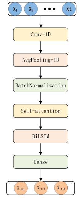
The input layer of the constructed generator network receives pre-processed data and employs a Convolutional layer for filtering operations to identify different features within the data. The Average Pooling layer reduces the size of feature maps by selecting the average value in each sub- region, thus reducing the number of network parameters, lowering computational costs, and helping to reduce over-fitting. The Batch Normalization layer improves the training speed and performance of deep neural networks, enhancing the model’s robustness and generalization capability, and reducing over-fitting. The Self-Attention layer learns more effective feature representations, enhancing the model’s expressive power and generalization ability, resulting in improved prediction accuracy and efficiency. The Bidirectional LSTM layer processes input sequences simultaneously in both forward and backward directions, capturing relationships within the sequence more effectively. The Dense layer performs linear transformations on the data, followed by nonlinear activation, further enhancing the model’s expressive power. Finally, the data is flattened into a one-dimensional vector, and the output layer produces the model’s prediction results. The generator network structure is illustrated in Figure 1.
Discriminator
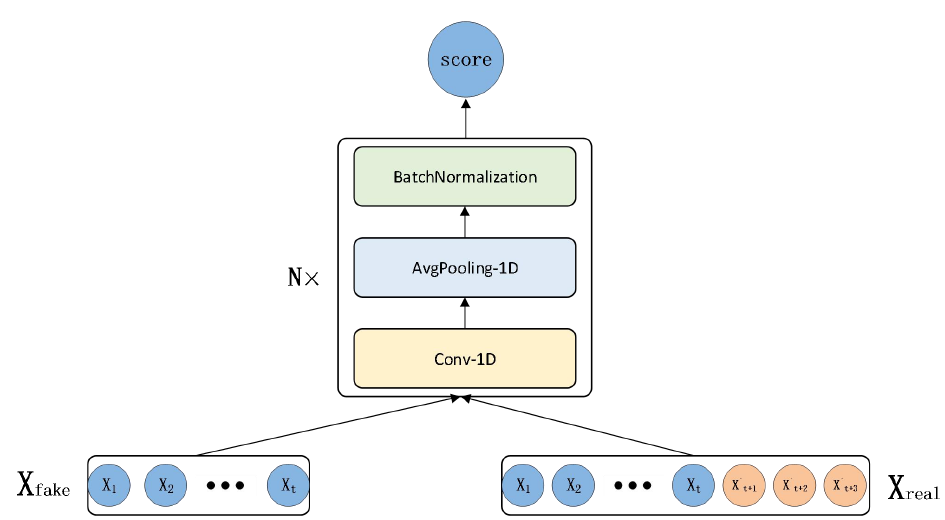
The discriminator network of the proposed model processes input data, which combines generated stock closing prices from the generator with real stock closing prices. This approach aims to increase the length of the input data and enhance the discriminator’s accuracy in learning classification.
The convolutional layer plays a crucial role in enabling the model to learn valuable features from both real stock data and generated predicted stock data, contributing to improved classification accuracy. Following the convolutional layer, the average pooling layer reduces the dimensionality of the output, eliminating unnecessary information and enhancing the model’s robustness and generalization capability.
To ensure robustness and stability, the batch normalization layer normalizes the output from the average pooling layer, mitigating issues such as gradient vanishing or exploding. In this study, three CNN units, each comprising a convolutional layer, an average pooling layer, and a batch normalization layer, are selected to reinforce the discriminator’s performance. Their primary function is to discern the authenticity of input data, determining whether the data is derived from the real dataset or generated by the The discriminator’s output is a scalar value (score) ranging between 0 and 1, with a score closer to 1 indicating that the input data closely resembles real data. The structure of the discriminator network is illustrated in Figure 2.
generator.
Build CAL-WGAN-GP Model
The combined generator and discriminator networks described above constitute the CAL-WGAN-GP model proposed in this study. The training process of the model follows these steps:
Step 1: Initialize the weights of the generator and discriminator networks.
Step 2: Iterative Training: • In the discriminator network, train the discriminator using real data samples to obtain the error on the real data. Then, train the discriminator using a mixture of fake data samples generated by the generator and real data samples to obtain the error on the generated data. Apply gradient penalty to constrain the difference between these two errors, resulting in the discriminator’s error. Finally, update the discriminator’s parameters using gradient descent based on this error.
- In the generator network, train the generator using the generated data to train the discriminator network. Update the generator’s parameters based on the error provided by the discriminator network.
- To eliminate fake gradients and enable the generator to generate higher-quality data, train the discriminator network once while training the generator network multiple times. In this study, the value of n, which represents the number of times the generator network is trained for each training of the discriminator network, is set to 3.
Step 3: Repeat the above Step 2 until the model converges.
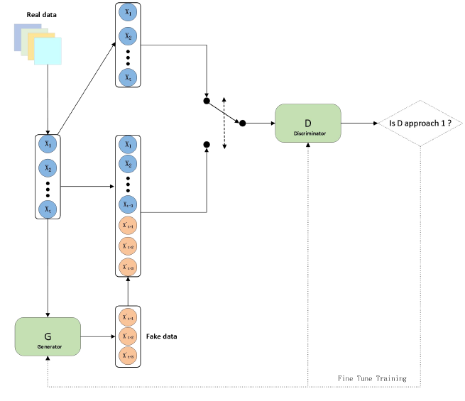
The structure of CAL-WGAN-GP is illustrated in Figure 3. This study begins by pre-processing the dataset and then employs the training process of the described model on the pre-processed data. Finally, the model computes gradient penalties, updates gradients, and consequently updates the parameters of both the discriminator and generator networks to achieve convergence.
The loss function of CAL-WGAN-GP is based on the loss function of WGAN-GP. The loss function of WGAN-GP replaces the Jensen-Shannon divergence with the Wasserstein distance. Unlike the optimization objective of the original GAN, the optimization goal of WGAN is to minimize the distance between the probability distributions of real data and generated data.
Its loss function consists of three components: 1. Generator’s loss function: This part of the loss function is the same as the original WGAN, aiming to maximize the Wasserstein distance between samples generated by the generator and real samples. 2. Discriminator’s loss function: This part of the loss function is also the same as WGAN, aiming to minimize the Wasserstein distance between real samples and generator samples. 3. Gradient penalty term: This is a new feature of WGAN- GP, which adds an additional regularization mechanism to the discriminator’s loss function to constrain the weight distances. Specifically, when calculating the Wasserstein distance between real samples and generator samples, a penalty is applied to the gradients, making the gradients of the discriminator with respect to generator samples smoother. This helps avoid erroneous adversarial training between the generator and discriminator and improves the efficiency of the generator in generating data.
The mathematical expression of the loss function is shown in equation (1).
[ ] [ ] ( ) ˆ
ˆ ˆ ˆ ( ) (z) x ( ) 2 ˆ ( ) ( ( )) ( ) 1 data z x WGAN GP x p x z p p x x L E f x E f G z E f x λ − = − + ∇ −
2 (1) In the equation, ( ) f x represents the output of the discriminator for real sample x , ( ( )) f G z represents the output of the discriminator for generated sample ( ) G z , ˆx is a random linear interpolation between real and generated samples, λ is a hyper parameter, ( ) data P x and (z) zP are the probability distributions of real data and the prior distribution in the latent space, and G(z) is the generator function.
Experiments
Dataset
The daily stock dataset of China Ping An (sh.601318) from the Shanghai Stock Exchange encompasses a variety of features, including opening price, closing price, highest price, lowest price, trading volume, percentage change, and more. These features, extensively employed in related literature [28], provide rich information for predictive models, rendering the dataset highly valuable for research purposes.
For this study, daily stock data from China Ping An, a listed company on the Shanghai Stock Exchange (sh.601318), was selected. To facilitate the model in more accurately capturing hidden information within the data, the study incorporated features defined in the method and constructed the China Ping An stock dataset. Additionally, daily stock data from other insurance companies within the same industry as China Ping An, such as China Life (sh.601628), New China Insurance (sh.601336), and Pacific Insurance (sh.601601), were selected. These datasets were constructed using the same data processing methods.
Data for this experiment was downloaded using the baostock package in Python, covering the time period from January 4, 2012, to December 30, 2022. As stock market data is not updated during market holidays, the dataset excludes data for weekends or holidays. The number of data points in each stock dataset is 2621.
Given that stock data is collected sequentially over time and represents two-dimensional data, but neural networks require three-dimensional input, a sliding window approach with a window size of 30 was employed. This transformation converted the two-dimensional data into three dimensions, representing the total data samples (samples), the length of the sliding window (time-steps), and the number of stock features (features). Subsequently, the transformed data, post sliding window processing, was split into a training dataset and a testing dataset in chronological order. The first 70% of the data served as the training set for model training, while the remaining 30% constituted the testing set for analysing and evaluating the model’s prediction performance.
The training set comprises 1885 data points (the first 70%), and the testing set consists of 786 data points (the last 30%). Following sliding window processing, the shape of the training dataset is (1835, 30, 25), and the shape of the testing dataset is (786, 30, 25).
Data Pre-Processing
In the original dataset, there might be instances of missing values or corrupted data. As a preliminary step, the experiment replaces these missing values or corrupted data with zeros. Substituting missing values or corrupted data with zeros serves to standardize the input dataset, facilitating subsequent data processing and analysis.
In stock data, variables like stock opening prices, highest prices, lowest prices, etc., are price data, while trading volume is quantitative data. Technical indicators also have different units of measurement. Inputting unprocessed data into the model can introduce certain disturbances in the prediction results due to differences in data units. To eliminate the influence of these disparities in data units, this experiment applies the Min Max Scalar function from the Sklearn. Pre-processing library to normalize the data. This normalization process ensures that all data are within a consistent numerical range. As a result, the input features of stock data become more effective and accurate, enhancing the model’s ability to predict stock data. The formula for data normalization is shown in equation (2) min max min x x xscaled x x − = − (2) In the equation, x represents the original data, xscaled represents the normalized data, x𝑚i𝑛 represents the minimum value in the original data, and xmax represents the maximum value in the original data.
Evaluation Indicators
To comprehensively assess the predictive capability of the model from different perspectives, the experiment employs four evaluation metrics to quantify model performance. These metrics include Root Mean Squared Error (RMSE), Mean Absolute Error (MAE), Mean Absolute Percentage Error (MAPE), and R-squared coefficient (R^2). The formulas for calculating these four metrics are as shown in equations (3) to (6):
1 ˆ
n t t t M A E x x n = = − ∑ (3)
1
1 ˆ ( )
n t t t RMSE x x n = = − ∑
2 (4)
1 ˆ 100% n t t
x x MAPE n x =
− = ∑ (5)
1 t t n ∑
2 ˆ
x x R x x − = −
t t t n
2 1 = (6) ∑
2 t t t
1 = In the equation, ˆtx represents the model’s predicted result, tx represents the actual values in the dataset, tx represents the average value of tx , and n represents the total number of data points in the dataset.
MAPE (Mean Absolute Percentage Error) represents the relative error between predicted values and actual values. A lower MAPE indicates a smaller error between predicted and actual values, signifying more accurate predictions. RMSE (Root Mean Squared Error) is used to assess the extent of error between predicted values and actual values. It reflects the deviation between predicted and actual values, with smaller RMSE values indicating lower model bias and better model performance. MAE (Mean Absolute Error) measures the mean absolute value of the errors between actual values and predicted values. Smaller MAE values suggest relatively more accurate predictive performance by the model. R2 (R-squared) coefficient is employed to gauge the correlation between predicted values and actual values. The closer R2 is to 1, the stronger the model’s predictive capability, indicating its ability to accurately reflect the characteristics of the sample population.
Baseline Methods
To validate the stock prediction method proposed in this experiment and assesses its ability to enhance prediction accuracy, several baseline models were chosen for comparative experiments. Below, we provide an overview of the structures and relevant parameters of each model.
LSTM: The LSTM network comprises two layers of Long Short-Term Memory (LSTM) layers. The number of neurons in each layer is configured as 21 and 49, respectively. Following the LSTM layers, there is a fully connected layer with 43 neurons, and finally, an output layer with 3 neurons. GRU [29]: The GRU model consists of 2 layers of Gated Recurrent Unit (GRU) networks. The number of neurons in each layer is set to 75 and 157, respectively. Following these GRU layers, a fully connected layer with 187 neurons is concatenated, and subsequently, an output layer with 3 neurons is added. CNN-LSTM: In the CNN-LSTM model, a one-dimensional convolutional neural network (1D CNN) is configured with an output dimension of 157. The size of each one-dimensional convolutional kernel window is set to 2, and the same data padding method is employed. Subsequently, the data passes through a one-dimensional average pooling layer with a pooling window size of 2. The output data from this layer is then fed into an LSTM network. The LSTM network has 60 neurons. Following the LSTM layer, there is a fully connected layer with 130 neurons. Finally, the output layer is configured with 3 neurons. Basic WGAN-GP: In the Basic WGAN-GP model, the configuration of the discriminator network, loss function, and learning rate aligns with that of the CAL-WGAN-GP model. However, the generator network in the Basic WGAN- GP model is set as the aforementioned GRU network.
Experimental Environment and Parameter Settings
The CAL-WGAN-GP model and the baseline models were both constructed and executed in a 64-bit Windows 11 operating system, utilizing identical hardware and software environments. The essential hardware and software configuration details are provided in Table 1.
| Software/Hardware | Configuration |
|---|---|
| CPU | AMD 5800H |
| GPU | RTX 3050 |
| Python | 3.7.16 |
| Tensor flow | 2.4.0 |
| CUDA | 11.1 |
| Keras | 2.4.3 |
| Numpy | 1.19.3 |
| Pandas | 1.3.5 |
| Scikit-learn | 0.22.1 |
| Matplotlib | 3.4.0 |
Table1: Software and hardware configuration.
In order to optimize the prediction performance of the model, this experiment uses the whale optimization algorithm and multiple repeated experiments to determine various parameters of the model, such as the learning rate, the number of neurons, and the number of network layers. According to the changes in the loss curve, each baseline model is trained for 100 rounds, the CAL-WGAN-GP model is trained for 230 rounds, and the data batch size is set to 128.
To optimize the predictive performance of the models, this experiment utilized the Whale Optimization Algorithm and conducted multiple repetitions to determine various model parameters such as learning rates, the number of neurons, and network layers. Based on the changes in the loss curves, all baseline models were trained for 100 epochs, while the CAL-WGAN-GP model was trained for 230 epochs, with a batch size set to 128.
The Adam optimizer has been proven to be one of the most effective optimizers for training neural networks [30]. Its key feature is its ability to adaptively compute the learning rate and momentum for each weight, thereby helping the generator and discriminator networks achieve a better balance in learning and avoiding the issues of gradient explosion or vanishing. Since the generator and discriminator play distinct roles in the model, the learning rate settings differ slightly. In the generator network, the learning rate is set to 0.0001, allowing for slower learning of the data distribution and the generation of more accurate samples. In
the discriminator network, the learning rate is set to 0.0004, which enables faster learning for improved discrimination between real and fake samples. Similarly, the optimizers for all baseline models are also set to use the Adam optimizer.
Stock market prices are influenced by multiple factors, necessitating the consideration of various variables and their interactions when predicting future trends. Employing a multi-step forward prediction approach, the model utilizes historical data for incremental forecasting and adjustments, thereby enhancing its predictive capabilities and reducing prediction errors. In the experiments, the historical window size was set to 30, while the future window size was set to 3. This means that the model predicts the stock trends for the next 3 days based on historical data from the past 30 days. By observing the model’s prediction results, investors can gain insights into market trends and changes, allowing them to make informed decisions.
Analysis of Experimental Results
The CAL-WGAN-GP model endeavors to predict the closing prices of China Ping An, China Life, New China Insurance, and Pacific Insurance stocks by leveraging insights gained from their historical data. Comparative evaluations are conducted against baseline models, including LSTM, GRU, CNN-LSTM, and Basic WGAN-GP. To enhance the robustness of the experimental findings, each model undergoes five repetitions of experiments on the test dataset, and the results are averaged to mitigate potential errors.
Table 2 presents a comprehensive comparison of CAL- WGAN-GP with various baseline prediction models on the test datasets of China Ping An, China Life, New China Insurance, and Pacific Insurance. The bolded data in the table signifies the best test results achieved for each respective dataset. In an effort to offer a more tangible depiction of the experimental outcomes and their alignment with real stock data, a fitting evaluation is performed on any continuous 100 trading days selected from the same experiment for the test datasets of China Ping An, China Life, New China Insurance, and Pacific Insurance.
Visual representations in Figures 4-7 are designed to enhance clarity in observing the experimental results and assessing the conformity of model predictions with actual stock closing prices. In these graphs, the horizontal axis represents the prediction data for 100 trading days spanning from the 400th to the 500th day within the test dataset, while the vertical axis illustrates the closing prices of the stocks. This graphical presentation facilitates a more insightful examination of the model predictions in relation to the observed stock closing prices.
| Evaluation index | LSTM | GRU | CNN-LSTM | WAGN-GP | CAL-WAGN-GP | |
|---|---|---|---|---|---|---|
| Ping An of China | MAPE | 5.604 | 4.89 | 6.214 | 4.042 | 3.083 |
| RMSE | 3.851 | 4.208 | 4.18 | 3.233 | 2.615 | |
| MAE | 3.434 | 3.235 | 3.779 | 2.437 | 2.004 | |
| R2 | 0.936 | 0.952 | 0.927 | 0.963 | 0.973 | |
| China Life Insurance | MAPE | 7.014 | 10.11 | 8.572 | 11.809 | 6.453 |
| RMSE | 2.91 | 4.179 | 3.437 | 4.982 | 2.699 | |
| MAE | 2.498 | 3.636 | 3.071 | 4.299 | 2.175 | |
| R2 | 0.751 | 0.567 | 0.664 | 0.118 | 0.922 | |
| New China Insurance | MAPE | 7.434 | 6.626 | 7.507 | 8.411 | 5.152 |
| RMSE | 3.943 | 4.672 | 4.242 | 4.693 | 2.699 | |
| MAE | 3.48 | 3.376 | 3.573 | 3.963 | 2.279 | |
| R2 | 0.876 | 0.873 | 0.867 | 0.811 | 0.922 | |
| Pacific Insurance | MAPE | 6.23 | 6.149 | 6.809 | 8.85 | 5.007 |
| RMSE | 2.353 | 2.665 | 2.561 | 3.431 | 1.915 | |
| MAE | 2.005 | 2.003 | 2.196 | 2.858 | 1.472 | |
| R2 | 0.87 | 0.865 | 0.848 | 0.699 | 0.876 |
Table 2: The prediction performance of each model in the four stock data sets.
Analysing the outcomes presented in Table 2, it is evident that the R2 coefficient predicted by each model closely approximates 1, indicating a strong fitting effect. The CAL-WGAN-GP model outperforms the compared baseline models (LSTM, GRU, CNN-LSTM, and Basic WAGN-GP) across metrics such as MAPE, RMSE, and MAE, showcasing superior predictive accuracy. Specifically, in comparison to the baseline models, the CAL-WGAN-GP model exhibits an average increase of 40.8%, 35.2%, and 42.9% in MAPE, RMSE, and MAE, respectively, on the China Ping An dataset. On the China Life dataset, the average increases are 28.5%, 27.4%, and 32.9%, respectively. For the Xinhua Insurance dataset, the predicted MAPE, RMSE, and MAE experience an average increase of 30.7%, 38.1%, and 36.4%, while the Pacific Insurance dataset sees an average increase of 27.0%, 29.0%, and 33.6%, respectively.
In summary, the CAL-WAGN-GP model consistently outperforms the baseline models across all four datasets, demonstrating its accuracy and robust predictive capabilities. It stands out as an effective model for forecasting the closing prices of insurance stocks, providing valuable insights for investors to make informed and precise investment decisions.
Observing Figures 4-7, it is noticeable that there exists a certain degree of error in the fitting curves of various models when compared to the actual trends in stock data. However, these fitting curves generally capture the overall trend in real stock closing prices. Notably, CAL-WGAN-GP exhibits fitting curves that closely align with the actual trends in stock closing prices, indicating its superior ability to make accurate predictions of stock closing prices.
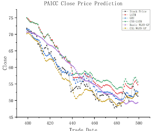
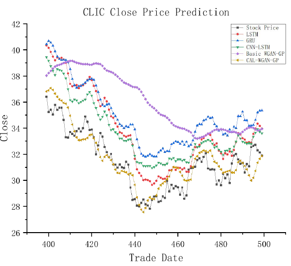
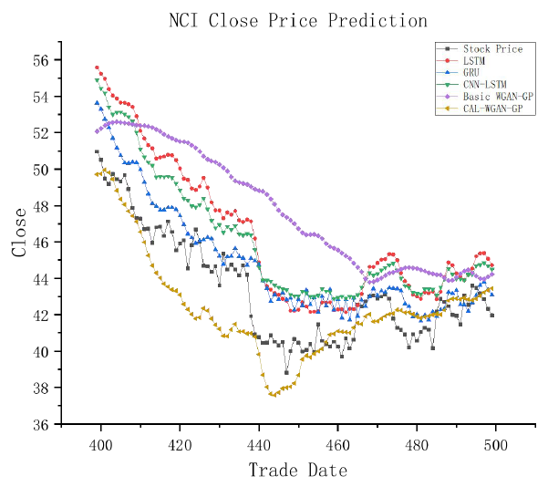
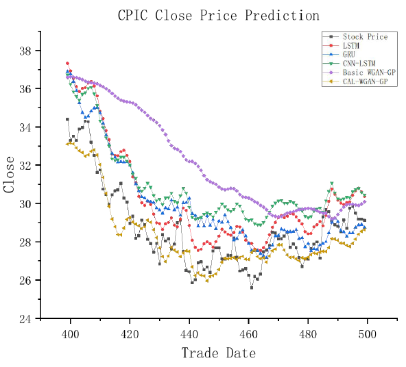
Figure 7: Partial 100-day fitting graph of the Pacific Insurance test set. Conclusion This paper introduces an innovative approach, CAL- WGAN-GP, designed for predicting closing prices in the insurance industry’s stock market. Employing a data generation strategy, this method enhances data quality and stock price prediction accuracy by integrating a self- attention mechanism and a CNN-BiLSTM model into the generator network.
models for accurate stock price prediction.
In future research endeavors, we plan to investigate the impact of additional data features and model parameters on stock data prediction. Additionally, we aim to explore the model’s generalization capabilities across a more extensive array of stock datasets.
Conflict of Interest
We have no conflict of interests to disclose and the manuscript has been read and approved by all named authors.
Acknowledgments
This work was supported by the Philosophical and Social Sciences Research Project of Hubei Education Department (19Y049), and the Staring Research Foundation for the Ph.D. of Hubei University of Technology (BSQD2019054), Hubei Province, China.
References
-
Zhao T, Han Y, Yang M A Review of Time Series Data Prediction Methods Based on Machine Learning. Journal of Tianjin University of Science and Technology 36(5): 1-9.
-
Takahashi S, Chen Y, Ishii K (2019) Modeling Financial Time-Series with Generative Adversarial Networks. Physica A: Statistical Mechanics and its Applications 527: 121261.
-
Romero RAC (2018) Generative Adversarial Network for Stock Market Price Prediction. CD230: Deep Learning, Stanford University, pp: 5.
-
Zhang K, Zhong G, Dong J, Wang S, Wang Y (2019) Stock Market Prediction Based on Generative Adversarial Network. Procedia computer science 147: 400-406.
-
Lin H, Chen C, Huang G, Jafari A (2021) Stock Price Prediction Using Generative Adversarial Networks. J Comp Sci 17(3): 188-196.
-
Yan DM, Li B Stock Price Prediction Research Based on Generative Adversarial Neural Networks. Computer Engineering and Applications 58(13): 185-194.
-
Liu YL, Zhao GL, Zou ZR, Shengting W (2022) Stock Price Prediction Method Based on Sentiment Analysis and GAN. Journal of Hunan University (Natural Sciences) 49(10): 111-118.
-
Sonkiya P, Bajpai V, Bansal (2017) A Stock price prediction using BERT and GAN. arXiv preprint Conference 17, Washington, USA.
-
Asgarian S, Ghasemi R, Momtazi S (2023) Generative Adversarial Network for Sentiment ‐ Based Stock Prediction. Concurrency and Computation: Practice and Experience 35(2): e7467.
-
Polamuri SR, Srinivas K, Mohan AK (2022) Multi-Model Generative Adversarial Network Hybrid Prediction Algorithm (MMGAN-HPA) For Stock Market Prices Prediction. Journal of King Saud University-Computer and Information Sciences 34(9): 7433-7444.
-
Goodfellow I, Pouget-Abadie J, Mirza M, Xu B, Warde- Farley D, et al. (2014) Generative adversarial nets. Advances in neural information processing systems 27.
-
Radford A, Metz L, Chintala S (2015) Unsupervised Representation Learning with Deep Convolutional Generative Adversarial Networks. arXiv preprint.
-
Isola P, Zhu JY, Zhou T, Alexei A (2017) Image-to-Image Translation with Conditional Adversarial Networks. Proceedings of the IEEE conference on computer vision and pattern recognition 1: 1125-1134.
-
Miyato T, Kataoka T, Koyama M, et al. (2018) Spectral Normalization for Generative Adversarial Networks. arXiv preprint.
-
Wang TC, Liu MY, Zhu JY, Tao A, Kautz J, et al. (2018) High- Resolution Image Synthesis and Semantic Manipulation with Conditional Gans. Proceedings of the IEEE conference on computer vision and pattern recognition: 8798-8807.
-
Arjovsky M, Chintala S, Bottou L (2017) Wasserstein Generative Adversarial Networks. International conference on machine learning 70: 214-223.
-
Gulrajani I, Ahmed F, Arjovsky M, Dumoulin V, Courville A (2017) Improved Training of Wasserstein Gans. Advances in neural information processing systems, pp: 1-11.
-
Vaswani A, Shazeer N, Parmar N, Uszkoreit J, Jones L, et al. (2017) Attention Is All You Need. Advances in neural information processing systems 30.
-
Donahue J, Hendricks LA, Guadarrama S, Venugopalan S, Guadarrama S, et al. (2015) Long-Term Recurrent Convolutional Networks for Visual Recognition and Description. Proceedings of the IEEE conference on computer vision and pattern recognition: 2625-2634.
-
Xu L, Ren JS, Liu CJ, Jia J (2014) Deep Convolutional Neural Network for Image Deconvolution. Advances in neural information processing systems 2: 1790-1798.
-
Hochreiter S, Schmidhuber J (1997) Long short-term memory. Neural computation 9(8): 1735-1780.
-
Mirjalili S, Lewis A (2016) The whale optimization algorithm. Advances in engineering software 95: 51-67.
-
Bentes C, Velotto D, Tings B (2017) Ship Classification in Terrasar-X Images with Convolutional Neural Networks. IEEE Journal of Oceanic Engineering 43(1): 258-266.
-
Medsker LR, Jain LC (2001) Recurrent neural networks. Design and Applications 5(64-67): 2.
-
Xu H, Xu B, Xu K An Overview of Machine Learning Applications in Stock Price Prediction. Computer Engineering and Applications 56(12): 19-24.
-
Shi Z, Hu Y, Mo G, Wu J (2022) Attention-Based CNN- LSTM and Xgboost Hybrid Model for Stock Prediction. arXiv preprint.
-
Li M, Ning DJ, Guo JC (2019) CNN-LSTM Model Based On Attention Mechanism and its Application. Computer engineering and applications 55(13): 20-27.
-
Wang Y, Guo YK (2019) Application of Improved Xgboost Model in Stock Forecasting. Computer Engineering and Applications 55(20): 202-207.
-
Shejul AA, Chaudhari A, Dixit BA (2023) Stock Price Prediction Using GRU, SimpleRNN and LSTM[M]/ Intelligent Systems and Applications: Select Proceedings of ICISA 2022. Singapore: Springer Nature Singapore 959: 529-535.
-
Kingma DP, Ba J (2014) Adam: A Method for Stochastic Optimization. arXiv.
- Revolutionizing Property Measurement Through Artificial Intelligence: The Journey of PropertyMeasure.ai
- AI Infused Business Model Innovation for Competitive Advantage in the Era of Big Data and Digital Transformation
- Use of CPM/PERT in the Effort to Eradicate Polio
- Integrated Multimodal Deep Learning Framework for Early Detection of Mouth Cancer Using CT Imaging and Clinical Symptom Analysis
- Artificial Intelligence in Medical Robotics and Assistance: An Overview
- Server Migration with Multipath-QUIC