Biomathematical Modeling in Clinical Intelligent Diagnosis and Treatment
Hemorrhagic stroke, a severe cerebrovascular disorder caused by the rupture of brain blood vessels, is characterized by high acute mortality rates and enduring neurological impairments. To provide more targeted clinical recommendations, this study, based on the clinical data of patients with hemorrhagic stroke, extensively explores the relationships between edema changes, treatment conditions, and modified Rankin Scale (MRS) scores. The HemExPred, EdemaVolReg, and PrognosisPred models are meticulously designed to address these three critical aspects. In this study, we skilfully employed machine learning techniques to identify characteristics associated with hematoma expansion events, with the effectiveness of the ElasticNet technique being particularly notable. Additionally, polynomial regression demonstrated exceptional fitting capabilities in deciphering the complexities of edema volume changes. Utilizing the ExtraTreesRegressor model, with an R^2 of 94.6% and 90.6%, we successfully predicted the future trajectories of patients, affirming that hematoma volume, edema volume, and age are key determinants of prognosis. Through in-depth analysis, this research provides valuable insights for clinical decision-making in hemorrhagic stroke, aiding physicians in devising more precise and effective treatment strategies.
Introduction
The pressing difficulty for our society to confront the intricacies and gravity of hemorrhagic stroke, a variant of cerebrovascular affliction [1]. This particular stroke manifestation, often characterized by its abrupt onset and rapid progression [2], engenders potential treatment delays and dangerous consequences that imperil the lives of afflicted individuals [3], as elegantly depicted in Figure
1. Historically, hemorrhagic stroke and its therapeutic interventions have grappled with many pivotal concerns [4], including hematoma expansion [5], edema, and prognostic evaluation [6].
Within the first 48 hours following the incursion of hemorrhagic stroke, patients may encounter the distressing occurrence of hematoma expansion and fluctuations in edema volume [7], engendering a formidable challenge in clinical management. Remarkably, hematoma dilatation and edema are pivotal factors that significantly shape the trajectory of this affliction, exerting a profound influence on patient prognoses [8]. Hematoma expansion can potentially exacerbate neurological impairment, while edema, by intensifying intracranial pressure, perpetuates further injury to delicate brain tissue. Thus, the effective monitoring and management of hematoma dilatation and edema emerge as critical imperatives, promising to ease the prognosis of hemorrhagic stroke patients [9]. To this end, medical practitioners and healthcare professionals employ the Modified Rankin Scale (MRS) score, which comprehensively assesses patients’ neurological impairments and self-care capabilities [10]. This score assumes paramount significance, serving as a pivotal gauge of the patient’s overall prognosis.
![Figure 1: Historically, hemorrhagic stroke and its therapeutic interventions have grappled with many pivotal concerns [4], including hematoma expansion [5], edema, and prognostic evaluation [6].](/fulltextimages/12010/fig_1.png)
In recent times, the convergence of medical imaging and the vast realm of big data analytics have orchestrated a profound transformation in stroke research and therapeutic interventions [11]. Notably, Xu Y, et al. [12] harnessed the potential of a deep learning approach to facilitate the discernment of computed tomography findings, thereby aiding in refined diagnostic endeavors. Likewise, the commendable contributions of Mattila OS, et al. [13] unveiled a pioneering screening methodology for acute hemorrhagic stroke, leveraging data derived from prehospital examinations. This amalgamation of cutting- edge technologies augments the precision of hemorrhagic stroke diagnosis and furnishes invaluable support in the realm of targeted treatment recommendations. By synergistically amalgamating medical imaging technology and the omnipotent prowess of big data analytics, healthcare professionals have enhanced capabilities to meticulously assess the propensity for hematoma expansion and edema [14]. This newfound understanding catalysis shaping tailored, individualized treatment plans [15], thus was engendering a palpable improvement in patient prognoses.
Undoubtedly, machine learning is a pivotal tool within the vast landscape of big data analytics [16], exerting a pervasive influence in hemorrhagic stroke research and therapeutic interventions [17]. Practitioners can leverage the immense potential of machine learning algorithms to glean invaluable insights from copious clinical data [18], unravelling concealed patterns and correlations that elude the naked eye. By scrutinizing an array of crucial variables encompassing clinical manifestations, imaging characteristics [19], treatment modalities [20], and predictive data about hemorrhagic stroke patients, machine learning bestows upon healthcare professionals an enhanced comprehension of the intricate intricacies inherent in this affliction, empowering them to deliver personalized and bespoke support while making treatment decisions. The harmonious integration of techniques drawn from medical imaging [21] and big data analytics [22] kindles within us the remarkable ability to facilitate the prognosis of patients grappling with hemorrhagic stroke. Armed with accurate diagnostic capabilities and individualized treatment plans [23], we can effectively mitigate the harmful impact of hematoma expansion and edema, elevating life quality and fostering notable functional recovery among afflicted individuals.
Indeed, the realm of hemorrhagic stroke treatment remains fraught with challenges. Yet, the amalgamation of machine learning and the vast expanse of big data analytics [24] holds immense promise in furnishing healthcare professionals with treatment recommendations marked by unparalleled accuracy [25], precision, and targeting [26]. This transformative synergy empowers medical practitioners to navigate the intricate nuances of this affliction with heightened efficacy, paving the path toward a more favourable prognosis for patients grappling with hemorrhagic stroke.
The primary objective of this study was to meticulously analyse authentic clinical data about the peril of hematoma expansion, the presence and progression of perihematoma edema, and the 90-day MRS scores in individuals afflicted with hemorrhagic stroke. Leveraging the wealth of clinical and imaging information, the study sought to unveil latent insights and concealed patterns, thereby facilitating a comprehensive examination of temporal alterations in hematoma volume edema volume and subsequently prognosticating the clinical trajectory of hemorrhagic stroke patients. The ultimate aim of this endeavor lies in advancing the frontiers of stroke management, fostering efficient healthcare practices, and ultimately enhancing the quality of patient care. We endeavoured to delve into the intricacies surrounding the occurrences of hematoma expansion, the temporal fluctuations in edema volume, and the prognostic implications for patients afflicted with hemorrhagic stroke.
The principal contributions of this article are delineated as follows: 1) Development of an innovative model named HemExPred, specifically designed for predicting the likelihood of hematoma expansion events in hemorrhagic stroke patients during the initial 48 hours. This model integrates a variety of advanced machine learning techniques and significantly enhances the accuracy of predicting hematoma expansion events by precisely analysing the patient's personal medical history and clinical data. 2) The construction of the PrognosisPred model aimed at forecasting the prognosis of hemorrhagic stroke patients. In the diverse array of machine learning algorithms utilized, the ElasticNet and ExtraTreesRegressor algorithms are particularly noteworthy, each exhibiting exceptional performance in their respective experimental settings. 3) This research also delves into data visualization and correlation analysis. Through these methodologies, we have extensively explored the impact of edema volume and hematoma volume on patient outcomes, offering new perspectives and practical guidance for the treatment and management of hemorrhagic stroke.
Method
**HemExPred**
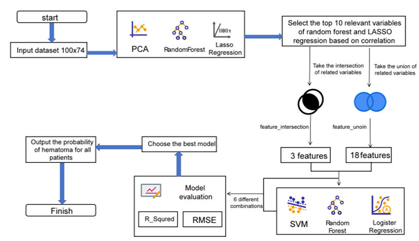
The endeavour, namely the Predictive Modeling of Hematoma Expansion Event Occurrence (HemExPred), aims to discern and forecast the likelihood of a hematoma expansion event transpiring. Drawing upon a comprehensive array of patient-specific factors, encompassing personal and disease history, time of onset, pertinent treatments, and imaging findings, HemExPred ingeniously calculates the probability of a hematoma expansion event (HEE) manifesting within 48 hours. In this research, we employ many feature extraction methodologies, including the techniques of principal component analysis, random forest, and lasso regression. By leveraging the potential of these methodologies, we meticulously extract the ten most pivotal features elucidated by each method, skilfully concatenating and intersecting them to form a robust feature set. Subsequently, these discerned features serve as the foundation for training support vector machine, random forest, and logistic regression models, which in turn bestow the ability to predict the probability of a hematoma expansion event occurring within the specified 48-hour window.
Let us allocate n follow-up visits for each patient, n∈[1,∞] allowing for any positive integer value. To determine the time interval, t, between each patient's follow-up examination and the onset of illness, we shall employ the following mathematical formula:
$$t = t_m + t_i - t_0 \quad i \in [1,n]$$
Here, $t_m$ represents the time interval between the onset and examination at the first visit, as indicated in Table 1. $t_i$ corresponds to the time point of examination at the i follow-up visit for the specific patient, while $t_0$ denotes the time point of examination at the first visit for that particular patient.
We have established specific criteria to define the event's occurrence, focusing on whether the hematoma volume exhibited notable changes within 48 hours of the patient's onset. To meet the criteria, any one of the following two conditions must be satisfied: (1) an absolute increase in volume greater than or equal to 6 ml, or (2) a relative increase in volume greater than or equal to 33%. To determine the occurrence of the event, we employ the following formula:
$$F \left( d_0, d_i \right)_{HEE} = \begin{cases} 1, & (d_i - d_0) > = 6 \text{ or } (d_i - d_0) \div d_0 > = 0.33 \\ 0, & \text{else} \end{cases}$$
Here, $d_0$ represents the volume of the clot at the first examination, while $d_i$ corresponds to the volume of the clot at the examination during the i follow-up visit. By evaluating the outcome of this formula, we can effectively determine whether the event of interest has taken place or not.
The illustrious flowchart of the HemExPred model, as depicted in Figure 2, shall serve as a visual representation of the steps as mentioned above. This diagram shall provide a comprehensive overview, guiding one through our model's intricate sequence of operations. The Random Forest algorithm, highlighted in references Schonlau M, et al. [27] and Wager S, et al. [28], is an effective classification tool in predictive modeling. It uses ensemble learning to create and merge multiple decision trees, providing a clear visual process that details the construction and synthesis of these trees for accurate predictions.
EdemaVolReg
This model, also known as EdemaVolReg, designed to analyse changes in edema volume over time, utilizes fitted regression models to construct regression curves that capture the dynamics of edema volume. By exploring the relationship between hematoma volume, volume of edema, and treatment, the researchers seek to unravel the intricate interplay between these factors.
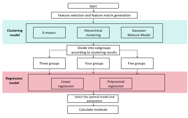
To accomplish this, the researchers embarked upon a series of steps. First, we diligently performed data cleaning, ensuring the integrity and reliability of the dataset. Feature matrices were constructed, serving as the foundation for training linear regression and polynomial regression models. The researchers conducted experiments using linear and polynomial regression models, aiming to identify the most suitable model and optimal parameters. Through rigorous analysis of the experimental results, we discerned the most appropriate model and parameter configurations, ensuring the accuracy and efficacy of their regression modeling endeavors.
Linear regression, an elementary statistical technique, serves as a foundational pillar in the realm of data analysis. It is expertly wielded to explore the intricate interplay between two variables, wherein one is designated as the dependent variable, often symbolized as y, while the other assumes the role of the independent variable, denoted as x.
$$ y = \beta_ {0} + \beta_ {1} x _ {1} + \beta_ {2} x _ {2} + \dots + \beta_ {p} x _ {p} + \dot {o} \tag {3} $$ The pursuit of linear regression lies in the quest for an optimal straight line, one that captures the essence of the relationship between these variables. Its purpose is to minimize the sum of distances, akin to errors, between the observed data points and the sublime trajectory of this line.
Polynomial regression, an extension of linear regression, serves as a formidable tool for encapsulating nonlinear associations present within datasets. Its fundamental premise involves augmenting the model by incorporating higher orders of the original features as novel attributes. Consequently, a meticulously tailored curve is fitted to the data, surpassing the limitations of a mere straight line.
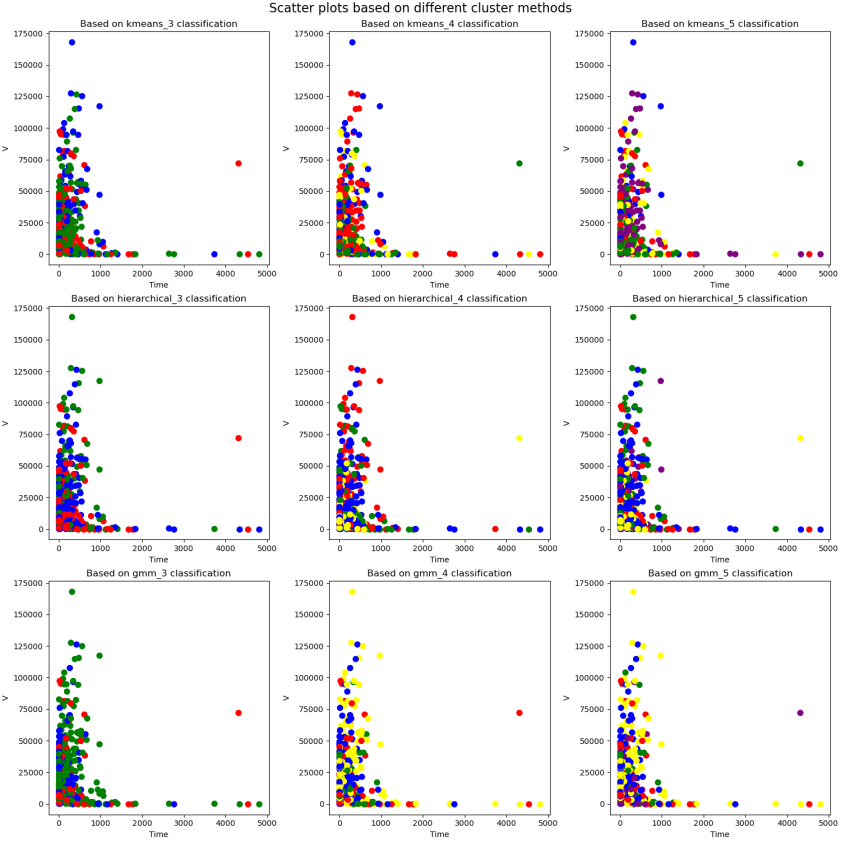
$$ y = \beta_ {0} + \beta_ {1} x _ {1} + \beta_ {2} x _ {2} ^ {2} + \dots + \beta_ {d} x _ {d} ^ {d} \tag {4} $$ It is imperative to embark upon a comprehensive exploration to delve into the intricate nuances of the evolutionary trajectory of edema volume in patients over time and its interindividual variations. In this regard, an initial prerequisite entails characterizing individual patients and unravelling potential divergent evolution paths. This scholarly endeavour undertakes a meticulous selection of pivotal patient features, subsequently employing a constellation of clustering algorithms, including K-means, hierarchical clustering, and Gaussian mixture models, to discern distinct patient subgroups.
With a dedicated focus on each patient subgroup, this study takes a stride forward by employing linear and polynomial regression models. These models fit the edema volume versus time curves for each subset. By harnessing the power of these models, explicit insights into the temporal trends of edema volume within each subgroup can be gleaned. The intricate procedural details are meticulously elucidated in Figure 3 below for comprehensive comprehension.
PrognosisPred
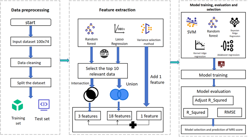
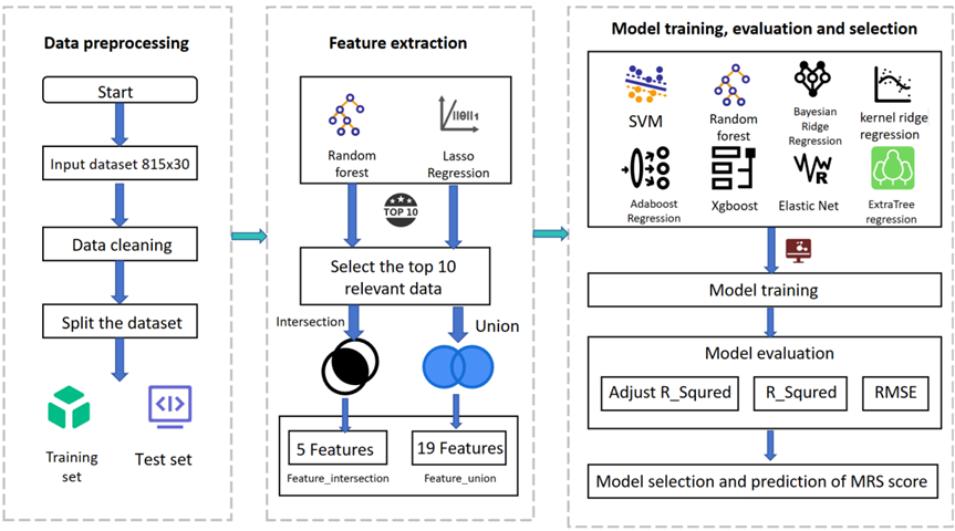
The Patient Prognosis Prediction Model (PrognosisPred) is a formidable tool to predict the outcome for patients afflicted with hemorrhagic stroke, drawing upon many influential factors. Following a patient’s initial consultation with a medical practitioner, wherein subsequent follow-up visits may occur, we employ two prediction schemes and construct two distinct models.
Firstly, PrognosisPredI considers solely the information gleaned during the patient’s inaugural visit to the doctor. This model focuses exclusively on the data obtained during this initial encounter to create a predictive framework. On the other hand, PrognosisPredII adopts a more comprehensive approach by amalgamating information derived from both patients’ visits. By incorporating and organizing the data from these two consultations, novel feature inputs are generated and subsequently employed for prediction. This holistic approach enables a more robust and nuanced prognosis evaluation.
These prediction schemes’ intricate mechanisms and intricacies are meticulously elucidated in Figure 4 and Figure 5, elegantly presented below for comprehensive comprehension.
ExtraTreesRegressor Reza M, et al. [29] is an exemplary ensemble learning method rooted in decision trees. It represents a specialized implementation of the ExtraTrees algorithm tailored for addressing regression tasks. The foundational workflow of ExtraTreesRegressor is elegantly delineated below. Before constructing the ExtraTreesRegressor model, it becomes imperative to establish a random subset to ascertain the number of decision trees (n_estimators) and the maximum depth (max_depth) of each tree. Subsequently, for every tree within the ensemble, a random subset is meticulously crafted by employing a process of random sampling with replacement from the original training set.
Within the realm of random feature selection, utilizing a random subset necessitates the random selection of a subset of features for training each decision tree. This stochastic feature selection process mitigates bias and bolsters the model’s diversity. Typically, the number of elements employed for each decision tree is regulated by the hyper parameter known as max_features, which can be defined as a fixed number of features or expressed as a percentage of the total feature set.
The decision trees are then forged based on the aforementioned random subset and random feature selection techniques, with each tree being trained on its respective random subset. During training, the decision tree partitions the feature space into distinct regions, guided by a designated splitting criterion (e.g., most minor square deviation). This partitioning process aims to minimize the variability of the prediction target, thereby ensuring optimal predictive performance.
$$H(X) = -\sum \log[P(x)]H(x)$$ (5)
Where denotes the entropy $P(x)$: denotes the probability that event $x$ occurs.
Harmonizing the predictions obtained from multiple decision trees is an integral step within the realm of ExtraTreesRegressor. Upon the culmination of training for each decision tree, the ExtraTreesRegressor algorithm artfully amalgamates their individual prediction outcomes for regression quandaries. This amalgamation takes the form of an average, where the predictions from each decision tree harmoniously converge to yield the ultimate prediction outcome. In the context of regression conundrums, the final prediction result materializes through the calculated average of the prediction results from each decision tree. This process can be succinctly encapsulated by the following formula:
$$y_{\text{pred}} = \frac{1}{n} \times \sum_{i=1}^{n} y_i$$ (6)
Where $n$ denotes the number of decision trees and $y_i$ denotes the prediction result of each decision tree.
The fundamental tenet that underlies ExtraTreesRegressor lies in imbuing each tree with a distinctive essence. Achieving this is accomplished through constructing multiple decision trees, while ingeniously introducing an element of randomness during the training process. This deliberate injection of randomness serves a twofold purpose: mitigating variance and elevating the model’s resilience and steadfastness.
**Experiments**
**Datasets**
The dataset emanates from the rich troves of data from Question E of the esteemed 20th China Graduate Student Mathematical Modeling Competition, fondly known as the "Huawei Cup." This dataset comprises five distinct tables, each offering a unique facet of information. Table 1 stands as a repository of patients’ comprehensive profiles, encompassing their details, medical history, and treatment regimens. Table 2, on the other hand, encapsulates the vivid realm of patient imaging information, explicitly of hematoma and edema volumes and their corresponding locations. Lastly, Table 3 unveils the intricate nuances of shape and grayscale distribution concerning the patients’ imaging information concerning hematoma and edema, thereby presenting a comprehensive compendium of insights for each image.
**Pre-Processing**
The tabular data, harnessed by invoking the Pandas library in Python, underwent a thorough analysis, revealing a pristine state untainted by missing values, outliers, or multicollinearity. Thus, it remained unadulterated and unaltered in its original form. In order to delve into the inquiry of whether follow-up information exerts an influence on the model’s predictions, two distinct data pre-processing techniques were employed to explore this profound query.
The first kind of data table, aptly christened “PreOne,” entailed constructing a predictive model devoid of the patient’s follow-up information. In this approach, the table was systematically segmented, one entry at a time, based on the ascending order of each image’s running number. Consequently, a tapestry of insights emerged, enabling an investigation into the interplay between the patient’s initial examination and the subsequent follow-up visits.
The second kind of data table, “PreTwo,” sought to establish a cohesive connection between the patient’s initial examination and the subsequent follow-up visits. Recognizing that merely correlating the first examination with the first follow-up visit would not optimally utilize the available data, this approach skilfully orchestrated a chronological correlation of the patient’s two examinations, regardless of whether they were the initial encounters. The ultimate objective was to discern the intricate correlation and interdependence between the two examinations.
Notably, the variable denoting sex underwent a distinctive encoding scheme, adopting a one-hot encoding methodology. Specifically, male and female genders were denoted by the values 0 and 1, respectively. Furthermore, the column of blood pressure was partitioned into two distinct columns, meticulously capturing the highest and lowest blood pressure readings. These columns were aptly designated as “Blood Pressure High” and “Blood Pressure Low,” respectively, enhancing the granularity and comprehensibility of the dataset.
**Correlation Analysis**
Pearson’s correlation coefficient, a statistical measure elucidated [30], serves as a metric to gauge the linear interplay between two numerical variables. Spanning a scale that ranges from -1 to 1, this coefficient manifests as a numerical reflection of the association between the variables under scrutiny.
The Spearman rank correlation method endeavors to evaluate the degree of association between two variables by considering the ordinal ranking of the data [31]. Unlike the unprocessed numerical values, this statistical approach duly acknowledges the significance of the variables’ rank order.
Kendall’s correlation Lin J, et al. [32], a nonparametric statistical technique, serves as a valuable tool for evaluating the correlation between two ordered data sets. The values yielded by Kendall’s correlation span the range of -1 to 1, where 1 signifies a perfect positive correlation, -1 indicates a perfect negative correlation, and 0 denotes the absence of any discernible correlation.
**Feature Extraction**
Principal Component Analysis (PCA) is a statistical methodology that condenses and streams data, there by effectuating its transformation into a novel set of uncorrelated variables known as principal components. These main components epitomize the directions that exhibit the highest variance within the initial dataset.
Random Forest-based feature extraction methodology primarily relies on the calculation of the esteemed Gini Index to determine the top ten features in terms of their importance for subsequent model training and prediction.
The loss function for Lasso regression is defined as follows:
$$L = L_{\text{quare}} + L_{\text{L1}}.$$
Where $L_{\text{quare}}$:
$$L_{\text{quare}} = \frac{1}{2n} \sum_{i=1}^{n} (y - X \times \beta)^2$$
$$L_{\text{L1}} = \alpha \times \sum |\beta|$$
In this formula, $n$ is the number of samples, $y$ is the target variable, $X$ is the identity matrix, $\beta$ is the characteristic coefficients, and $\alpha$ is the regularization parameter.
In the realm of Lasso regression and the random forest-based feature importance ranking method, it has come to light that the selected features do not invariably align within the same genre. Consequently, this paper has employed two distinctive feature extraction techniques. The first approach entails concatenating the elements acquired through both methods, thereby amassing a comprehensive set of features denoted as “feature union.” The second approach involves extracting ten features independently obtained from each method and subsequently identifying their intersection. This intersection of features is aptly referred to as “feature intersection.” By adopting these two feature extraction methodologies, this study aims to explore the potential synergies that arise from their combined utilization.
**Performance Evaluation Metrics**
The metric known as $R^2$ or the coefficient of determination, serves as a powerful indicator of the regression model’s proficiency in elucidating the fluctuations observed within the dependent variable. Spanning a range from 0 to 1, the $R^2$ value assumes its true potential in quantifying the model’s capacity to explicate the variability inherent in the said dependent variable. A higher $R^2$ value signals a superior ability of the model to account for and elucidate the intricate patterns and fluctuations within the dependent variable, thus enhancing our understanding of the underlying phenomena.
$$R^2 = 1 - \frac{\sum (y - \hat{y})^2}{\sum (y - \bar{y})^2}$$
Where $y$ is the true value, $\hat{y}$ is the predicted value, and $\bar{y}$ is the average of the true values.
$R_1^2$ is a correction to $R^2$ that takes into account the number of independent variables used in the model. Adjustment $R_1^2$ reflects the extent to which the independent variables explain the dependent variable, with values ranging from negative infinity to 1. $R_1^2$ larger value means a better fit.
$$R_1^2 = 1 - \left(1 - R^2\right) \frac{n - 1}{n - p - 1}$$
Where $n$ is the number of samples in the test set and $p$ is the number of features.
Root Mean Square Error (RMSE) and Mean Square Error (MSE) are metrics used to measure the prediction error of a regression model, both of which measure the average difference between the predicted and true values of the model. A smaller value of RMSE indicates a higher predictive accuracy of the model. Suppose there are $N$ samples, where the true value of the $i$ sample is $y^{(i)}$ and the predicted value is $\hat{y}^{(i)}$. The mathematical formulas for RMSE and MSE are:
$$\bar{y} = \frac{1}{n} \sum_{i=1}^{n} y_i$$
$$RMSE = \sqrt{\frac{1}{N} \sum_{i=1}^{N} \left(y^{(i)} - \hat{y}^{(i)}\right)^2}$$
$$MSE = \frac{1}{n} \sum_{i=1}^{n} \left(y_i - \hat{y}_i\right)^2$$
Experiment Settings
In the initial phase of the analysis, the dataset is partitioned into training and testing sets, adhering to an 8:2 ratio. Subsequently, feature extraction techniques, namely Principal Component Analysis (PCA), Random Forest, and Lasso Regression, are employed to identify the most influential ten features using each method. These selected features are then subjected to a concatenation and intersection process.
Three prominent metrics are employed to evaluate the relevance of the extracted main features: Pearson’s correlation coefficient, Spearman’s rank correlation coefficient, and Kendall’s correlation coefficient. Each of these metrics assesses the degree of correlation between the features. Features displaying high correlation are subsequently eliminated from consideration. Once this filtering process is complete, the remaining data is utilized to train a machine-learning model.
Results and Analysis
Statistical Analysis
Feature extraction is meticulously conducted on the PreOne dataset, wherein the feature variables undergo a meticulous screening process. Subsequently, the intersection and concatenation operations are deftly applied to glean the utmost value from these feature variables. Three paramount features are distilled from the intersection, while the concatenation yields a prodigious set of 18 salient features. A diverse array of machine learning techniques is employed to validate and predict. The comprehensive outcomes are eloquently presented in Table 1, which directly showcases the results of these experiments and the subsequent model validation. A discerning analysis reveals that the ElasticNet model surpasses all others in concatenation-on-based feature extraction. In contrast, the BayesianRidge model emerges as the preeminent choice for intersection-based feature extraction.
Curvilinear trajectories of edema volume throughout the temporal axis were adeptly fitted for each patient. Upon meticulous evaluation, it was determined that despite exhibiting elevated mean squared error (MSE) values, the simple linear model outperformed other models when polynomial regression calculations were applied. Allow me to provide you with the results:
$$ f (x) = 0. 0 0 0 1 x ^ {5} - 0. 0 0 0 1 x ^ {4} + 0. 0 0 0 1 x ^ {3} - 0. 2 1 0 2 x ^ {2} + 1 1 2. 9 5 5 9 x + 2 0 1 6 4. 9 7 2 2 $$ (14) The volumetric progression of edema, observed over a span of time, was meticulously modeled for all patients. Notably, amidst various modeling techniques, it was found that the simple linear model demonstrated superior performance despite exhibiting comparatively high MSE values when subjected to polynomial regression calculations. The results of the clustering are shown in Figure 6 below.
| Mould | R 2 1 | R2 | RMSE | ||||
|---|---|---|---|---|---|---|---|
| Feature Union | Feature Intersection | Feature Union | Feature Intersection | Feature Union | Feature Intersection | ||
| RandomForest Classifier | -1.9097 | -0.45485 | -0.30435 | -0.30435 | 0.48305 | 0.48305 | |
| SVR | -1.45173 | -0.22602 | -0.09905 | -0.09919 | 0.44341 | 0.44343 | |
| BayesianRidge | -1.20436 | -0.09855 | 0.01184 | 0.01509 | 0.42044 | 0.41975 | |
| KernelRidge | -1.48451 | -0.07416 | -0.11375 | 0.03696 | 0.44636 | 0.41506 | |
| XGBClassifier | -2.32537 | -1.07836 | -0.49068 | -0.86335 | 0.5164 | 0.57735 | |
| ElasticNet | -1.19677 | -0.10034 | 0.01524 | 0.01349 | 0.41972 | 0.42009 | |
| AdaBoost Classifier | -4.40373 | -0.66269 | -1.42236 | -0.49068 | 0.65828 | 0.5164 | |
| ExtraTrees Classifier | -2.32537 | -0.45485 | -0.49068 | -0.30435 | 0.5164 | 0.48305 | |
| Mould | Data | R 2 1 | R2 | RMSE | |||
| Feature Union | Feature Intersection | Feature Union | Feature Intersection | Feature Union | Feature Intersection | ||
| Random Forest Regressor | Pre One | -0.82903 | 0.03048 | 0.11702 | 0.13078 | 1.97107 | 1.95566 |
| Pre Two | 0.89758 | 0.87831 | 0.90471 | 0.88081 | 0.52916 | 0.59182 | |
| SVR | Pre One | -1.40779 | -0.29457 | -0.16238 | -0.16065 | 2.26152 | 2.25983 |
| Pre Two | -0.1448 | -0.0864 | -0.06504 | -0.06414 | 1.76908 | 1.76833 | |
| BayesianRidge | Pre One | -0.88932 | -0.22612 | 0.08792 | -0.09928 | 2.00329 | 2.19928 |
| Pre Two | 0.45086 | 0.276 | 0.48912 | 0.29084 | 1.22525 | 1.44356 | |
| Kernel Ridge | Pre One | -0.5771 | -0.06927 | 0.23864 | 0.04134 | 1.83029 | 2.0538 |
| Pre Two | 0.30232 | 0.25885 | 0.35093 | 0.27404 | 1.38105 | 1.46056 | |
| XGB Regressor | Pre One | -1.11766 | -0.15833 | -0.02232 | -0.03851 | 2.1209 | 2.13762 |
| Pre Two | 0.90231 | 0.89304 | 0.90911 | 0.89524 | 0.51679 | 0.55484 | |
| ElasticNet | Pre One | -0.58297 | -0.15011 | 0.23581 | -0.03113 | 1.8337 | 2.13002 |
| Pre Two | 0.31874 | 0.27491 | 0.3662 | 0.28977 | 1.3647 | 1.44465 | |
| AdaBoostRegressor | Pre One | -0.87111 | -0.08376 | 0.09671 | 0.02835 | 1.99361 | 2.06767 |
| Pre Two | 0.67697 | 0.48022 | 0.69948 | 0.49087 | 0.93973 | 1.22314 | |
| Extra Regressor | Pre One | -0.92804 | 0.02573 | 0.06922 | 0.12652 | 2.02372 | 1.96044 |
| Pre Two | 0.94172 | 0.90365 | 0.94578 | 0.90562 | 0.39916 | 0.52662 |
Table 1: Constructing a PrognosisPred Model Score Sheet Using PreOne and PreTwo Data
The study adopted the procedures outlined in Figures 4 & 5 employing various models such as Support Vector Machine, Random Forest Classification, BayesianRidge, KernelRidge, and AdaBoostRegressor to train the extracted features. The performance of these models was evaluated, as exemplified in Table 2. Notably, the KernelRidge model exhibited commendable performance on the PreOne dataset, albeit with a degree of uncertainty. Conversely, the ExtraTreesRegressor model demonstrated robust performance across a diverse range of scenarios on the PreTwo dataset, showcasing its generalizability.
Both experiments established significant correlations between the initial examination’s MRS scores, subsequent follow-up, and patient treatment. These findings surpassed the results obtained by pairing the examination data pairwise. Interestingly, the initial examination’s outcomes correlated more strongly with hematoma volume than the MRS scores. It is crucial for individuals with related medical conditions to consistently monitor their health and promptly seek medical attention when necessary.
Interpretability
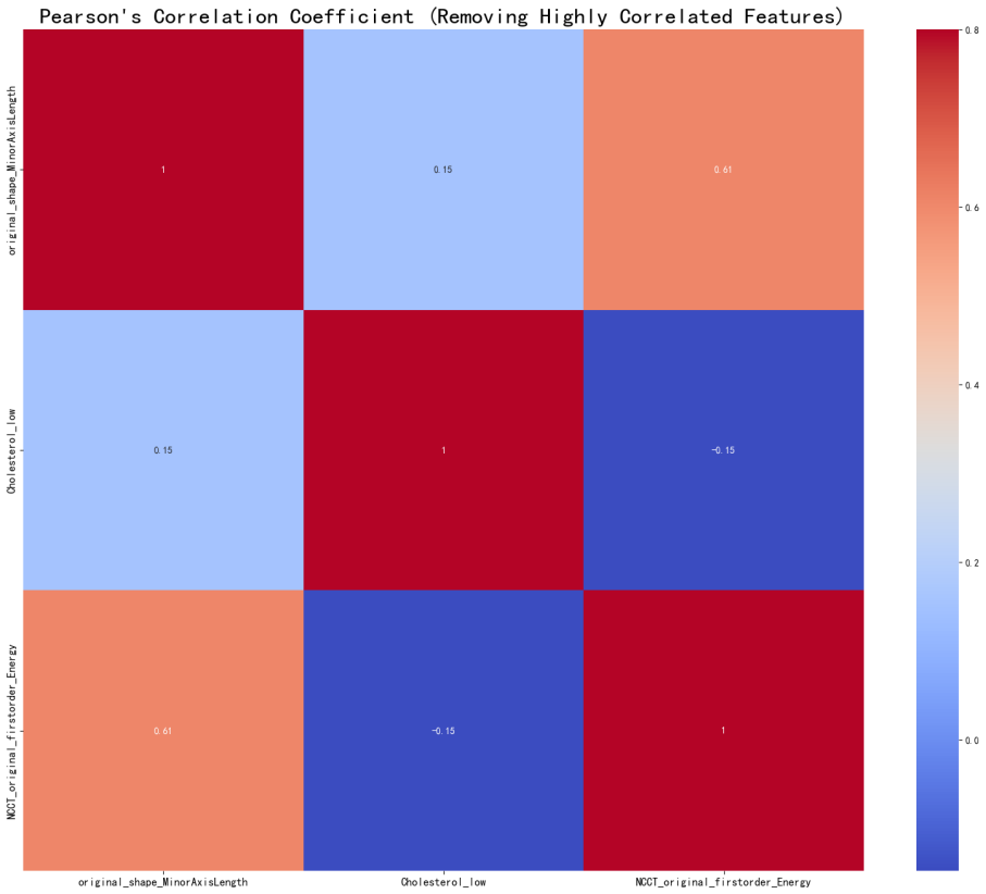
In determining the occurrence of hematoma expansion within a span of 48 hours, we sought to extract the features depicted in Figure 7 herewith, subsequently evaluating their similarity. It is evident that variables such as ‘age,’ ‘original_shape_Maximum2DDiameterColumn’, ‘original_ shape_Maximum2DDiameterRow’, ‘NCCT_original_ firstorder_10Percentile’, and ‘Cholesterol_low’ exhibit a positive correlation with prognostic MRS scores. Conversely, ‘Time between onset and first imaging,’ ‘original_shape_ LeastAxisLength,’ ‘original_shape_MinorAxisLength,’ and ‘Cholesterol_high’ demonstrate a negative correlation with prognostic mRS scores. Notably, ‘Cholesterol_low’ and ‘NCCT_original_firstorder_10Percentile’ emerge as indices of heightened significance, warranting attending physicians’ attention when tending to patients with a primary diagnosis.
Following the extraction of features from the ProTwo dataset, to generate the heatmap delineated in Figure 8 below, noteworthy observations come to light. Notably, variables such as ‘HM_ACA_L_Ratio_1’, ‘age,’ ‘original shape Elongation,’ ‘original shape Least-AxisLength,’ and ‘Cholesterol_low’ emerge as the top-ranked features in the Random Forest’s feature importance ranking. Remarkably, these results align harmoniously with the prior Lasso regression-based feature extraction outcomes. Furthermore, the Pearson correlation heatmap reveals certain intriguing associations. Specifically, a positive correlation is evident between ‘original_shape_ LeastAxisLength_2’ and ‘original_shape_MinorAxisLength_2’, while a negative correlation is observed between ‘NCCT_ original_firstorder_Minimum_2’ and ‘NCCT_original_-
firstorder_Minimum_2’. Noteworthy as well, ‘original_shape_ MajorAxisLength_1’ demonstrates a positive correlation with both ‘original_shape_Maximum2DDiameterSlice_1’ and ‘original_shape_Maximum2DDiameterRow_1’. These findings underscore the intricate interplay of variables within the dataset, shedding light on their respective relationships.
In our relentless pursuit to delve deeper into the intricate interplay between patients’ prognostic MRS scores at 90 days post-onset and the various facets of their disease and treatment-related information, alongside the outcomes of multiple imaging examinations, we have undertaken a comprehensive analysis. By scrutinizing the data, we aim to identify the factors that exhibit the strongest association with patients’ prognosis, facilitating more effective clinical diagnosis and treatment.
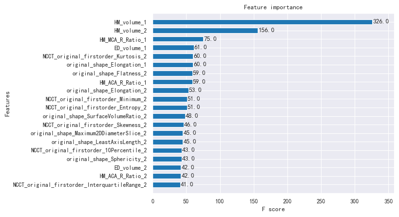
We have obtained the feature_union feature importance index through meticulous calculations, which serves as evidence of the rigor and accuracy of our model mentioned above. The analysis results are presented in Figure 8 below, providing valuable insights into the relative significance of the various features under consideration.
The profound exploration of the correlation between patients’ prognostic MRS scores at the 90-day mark following disease onset and a myriad of disease-related information, treatment-related details, and the outcomes of diverse imaging examinations has yielded compelling results. Notably, ‘HM_volume_1’, ‘HM_volume_2’, ‘HM_ MCA_R_Ratio_1’, ‘ED_volume_1’, and ‘HM_ACA_R_Ratio’ have emerged as highly correlated with the MRS as mentioned earlier scores in Figure 9. This finding validates the accuracy of influential factors, which exhibit significant correlations with prognostic mRS scores as determined through statistical analyses conducted within this study.
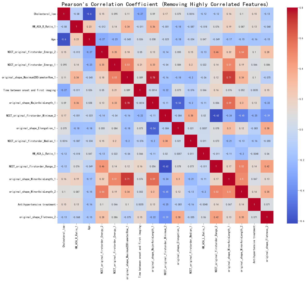
Figure 8: Heatmap of ProTwo data for feature extraction and correlation calculation Consequently, when conducting imaging assessments of patients afflicted with hemorrhagic stroke, it is imperative to direct our attention towards crucial indicators such as ‘HM_ volume,’ ‘ED_volume,’ ‘HM_MCA_R_Ratio,’ and ‘HM_ACA_R_ Ratio.’ The significance of ‘HM_volume’ outweighs other characteristics, underscoring its paramount association with a patient’s 90-day MRS score at the onset of the disease. Furthermore, based on the Pearson correlation coefficient, it becomes apparent that a positive correlation exists between ‘HM_volume’ and MRS scores. In simpler terms, larger values of ‘HM_volume’ correspond to higher MRS scores, indicating a more substantial hematoma volume and, subsequently, a poorer prognosis. It is worth noting that the presence of edema surrounding the hematoma contributes to further damage to brain tissue.
While ‘HM_MCA_R_Ratio’ and ‘HM_ACA_R_Ratio’ influence the progression, severity, and prognosis of hemorrhagic stroke, their specific etiology and mechanisms necessitate further investigation. In clinical diagnosis, it is crucial to diligently monitor changes in hematoma volume and prioritize research on therapeutic modalities or medications geared toward controlling it.
Discussion and Conclusion
This scholarly article undertakes a comprehensive examination in which both the PreOne and PreTwo datasets are subjected to training using a diverse array of models, including PCA and LASSO regression. Various feature extraction techniques, such as intersection and concatenation feature fusion, are employed to optimize the training process. Notably, the ExtraTreesRegressor model emerges as the top performer on the PreTwo dataset, exhibiting commendable scores across different feature fusion methods. Its superiority stems from its robustness in handling missing values and outliers, resulting in consistently higher scores than other models. This demonstrates the model’s potential for accurately predicting patients’ MRS scores based on multiple follow-ups.
However, it is crucial to acknowledge that the limited size of the dataset used in this study poses challenges for the KernalRidge model, which may exhibit underfitting or overfitting during training. To ensure the validity of its results, further datasets should be sought to validate the performance of this model.
Individuals afflicted with cerebral haemorrhage encounter substantial therapeutic challenges, particularly in the management of perihematomal edema. Recent developments have identified this condition as a potential focal point for therapeutic intervention. This study employs data modeling techniques to rigorously investigate these individuals’ essential prognostic factors and forecast their Modified Rankin Scale (MRS) scores. Nonetheless, the present research faces several constraints, including a restricted sample size, notably in studies incorporating cerebral magnetic resonance imaging (MRI), the absence of uniform metrics for evaluating edema severity and hematoma volume alterations, and a lack of prospective, novel data. A critical necessity exists for randomized controlled trials concentrating on the volumetric alterations in hematomas and edema. It is recommended that researchers utilize more sophisticated measurement methodologies to analyse high-quality imaging data, thereby facilitating an enhanced comprehension of the growth dynamics of hematoma and edema volumes. Such insights are imperative in the development of novel treatment strategies for individuals experiencing stroke.
Moving forward, future endeavors shall explore the essential features underlying the pathogenesis, diagnosis, and treatment processes in hemorrhagic stroke patients. By incorporating comprehensive information, the model can be refined to serve the medical field better, offering valuable diagnostic and treatment insights to physicians and patients alike, ultimately contributing to enhanced patient recovery.
Conflict of Interest
We have no conflict of interests to disclose and the manuscript has been read and approved by all named authors.
Acknowledgments
This work was supported by the Philosophical and Social Sciences Research Project of Hubei Education Department (19Y049), and the Staring Research Foundation for the Ph.D. of Hubei University of Technology (BSQD2019054), Hubei Province, China.
References
-
Doria JW, Forgacs PB (2019) Incidence Implications and Management of Seizures Following Ischemic and Hemorrhagic Stroke. Curr Neurol Neurosci Rep 19(7): 37.
-
Montano A, Hanley DF, Hemphill JC (2021) Hemorrhagic stroke. Handb Clin Neurol 176: 229-248.
-
Toyoda K, Yoshimura S, Nakai M, Koga M, Sasahara Y, et al. (2022) Twenty Year Change in Severity and Outcome of Ischemic and Hemorrhagic Strokes. JAMA Neurol 79(1): 61-69.
-
(2024) Risk factors for stroke recurrence in patients with hemorrhagic stroke Scientific Reports.
-
Ohashi SN, DeLong JH, Kozberg MG, Hart DJ, Veluw SJ, et al. (2023) Role of Inflammatory Processes in Hemorrhagic Stroke. Stroke 54(2): 605-619.
-
Chaudhary N, Pandey AS, Wang X, Xi G (2019) Hemorrhagic stroke Pathomechanisms of injury and therapeutic options. CNS Neurosci Ther 25(10): 1073- 1074.
-
Gu X, Li Y, Chen S, Yang X, Liu F, et al. (2019) Association of Lipids With Ischemic and Hemorrhagic Stroke A Prospective Cohort Study Among 267 500 Chinese. Stroke 50(12): 3376-3384.
-
Toyoda K, Yoshimura S, Nakai M, Minematsu K, Kobayashi S, et al. (2022) Twenty Year Change in Severity and Outcome of Ischemic and Hemorrhagic Strokes. JAMA Neurology 79(1): 61-69.
-
Broderick JP, Grotta JC, Naidech AM, Steiner T, Sprigg N, et al. (2021) The Story of Intracerebral Hemorrhage from Recalcitrant to Treatable Disease. Stroke 52(5): 1905-1914.
-
Bambhroliya AB, Donnelly JP, Thomas EJ, Tyson JE, Miller CC, et al. (2018) Estimates and Temporal Trend for US Nationwide 30-Day Hospital Readmission among Patients With Ischemic and Hemorrhagic Stroke. JAMA Netw Open 1(4): e181190.
-
(2024) Artificial intelligence with big data analytics based brain intracranial hemorrhage e-diagnosis using CT images. Neural Computing and Applications.
-
Xu Y, Holanda G, Souza F, Silva H, Gomes A, et al. (2021) Deep Learning Enhanced Internet of Medical Things to Analyze Brain CT Scans of Hemorrhagic Stroke Patients A New Approach. IEEE Sensors Journal 21(22): 24941- 24951.
-
Mattila OS, Ashton NJ, Blennow K, Zetterberg H, Harve Rytsala H, et al. (2021) Ultra Early Differential Diagnosis of Acute Cerebral Ischemia and Hemorrhagic Stroke by Measuring the Prehospital Release Rate of GFAP. Clinical Chemistry 67(10): 1361-1372.
-
Li X, Huang X, Tang Y, Zhao F, Cao Y, et al. (2018) Assessing the Pharmacological and Therapeutic Efficacy of Traditional Chinese Medicine Liangxue Tongyu Prescription for Intracerebral Hemorrhagic Stroke in Neurological Disease Models. Front Pharmacol 6(9): 1169.
-
Alex MRJ, Fernanda GSL, Regina SPC, Shirley MS, Garcia OS, et al. (2021) Prognostic molecular markers for motor recovery in acute hemorrhagic stroke A systematic review. Clin Chim Acta 522: 45-60.
-
Gu J, Shi Y, Chen N, Wang H, Chen T (2020) Ambient fine particulate matter and hospital admissions for ischemic and hemorrhagic strokes and transient ischemic attack in 248 Chinese cities. Sci Total Environ 715: 136896.
-
Ahangar AA, Saadat P, Heidari B, Taheri ST, Alijanpour S (2018) Sex difference in types and distribution of risk factors in ischemic and hemorrhagic stroke. Int J Stroke 13(1): 83-86.
-
Welten SJGC, Onland MNC, Boer JMA, Verschuren WMM, Schouw YT (2021) Age at Menopause and Risk of Ischemic and Hemorrhagic Stroke. Stroke 52(8): 2583- 2591.
-
Zhang T, Zhang W, Liu X, Dai M, Xuan Q, et al. (2022) Multifrequency Magnetic Induction Tomography for Hemorrhagic Stroke Detection Using an Adaptive Threshold Split Bregman Algorithm. IEEE Transactions on Instrumentation and Measurement 71: 1-13.
-
Lee EC, Ha TW, Lee DH, Hong DY, Park SW, et al. (2022) Utility of exosomes in ischemic and hemorrhagic stroke diagnosis and treatment. Int J Mol Sci 23(15): 8367.
-
Chen Y, Jiang C, Chang J, Qin C, Zhang Q, et al. (2023) An artificial intelligence based prognostic prediction model for hemorrhagic stroke. Eur J Radiol 167: 111081.
-
Nishimura A, Nishimura K, Kada A, Iihara K, (2016) Status and Future Perspectives of Utilizing Big Data in Neurosurgical and Stroke Research. Neurol Med Chir (Tokyo) 56(11): 655-663.
-
Ribeiro JAM, Salazar LF, Pacheco CR, Moreira SH, Oliveira S, et al. (2021) Prognostic molecular markers for motor recovery in acute hemorrhagic stroke: A systematic review. Clin Chim Acta 522: 45-60.
-
Feigin VL, Krishnamurthi RV, Parmar P, Norrving B, Mensah GA, et al. (2015) Update on the global burden of ischemic and hemorrhagic stroke in 1990-2013 the GBD 2013 study. Neuroepidemiology 45(3): 161-176.
-
Wang RC, Wang Z (2023) Precision Medicine Disease Subtyping and Tailored Treatment. Cancers 15(15): 3837.
-
Grzenda A, Widge AS (2024) Electronic health records and stratified psychiatry bridge to precision treatment. Neuropsychopharmacology 49(1): 285-290.
-
Schonlau M, Zou RY (2020) The random forest algorithm for statistical learning. The Stata Journal 20(1): 3-29.
-
Wager S, Athey S (2018) Estimation and inference of heterogeneous treatment effects using random forests. Journal of the American Statistical Association 113(523): 1228-1242.
-
Reza M, Haque MA (2020) Photometric redshift estimation using ExtraTreesRegressor Galaxies and quasars from low to very high redshifts. Astrophysics and Space Science 365(3): 50.
-
Mu Y, Liu X, Wang L (2018) A Pearson’s correlation coefficient based decision tree and its parallel implementation. Information Sciences 435: 40-58.
-
Farland TW, Yates JM (2016) Spearman’s Rank- Difference Coefficient of Correlation. In: MacFarland TW, et al. (Edn.). Introduction to Nonparametric Statistics for the Biological Sciences Using R. Springer International Publishing, pp: 249-297.
-
Lin J, Adjeroh DA, Jiang BH (2018) fastWKendall: an efficient algorithm for weighted Kendall correlation. Computational Statistics 33: 1823-1845.
- Revolutionizing Property Measurement Through Artificial Intelligence: The Journey of PropertyMeasure.ai
- AI Infused Business Model Innovation for Competitive Advantage in the Era of Big Data and Digital Transformation
- Use of CPM/PERT in the Effort to Eradicate Polio
- Integrated Multimodal Deep Learning Framework for Early Detection of Mouth Cancer Using CT Imaging and Clinical Symptom Analysis
- Artificial Intelligence in Medical Robotics and Assistance: An Overview
- Server Migration with Multipath-QUIC