Study on the Efficiency of China's Convertible Bond Market Based
on ARMA-GARCH Models

Bin Zhao* and Yi Wu

doi:10.23880/oajda-16000129

Open Access Journal of Data Science and Artificial Intelligence Research Article 17 min read

Study on the Efficiency of China's Convertible Bond Market Based on ARMA-GARCH Models

Bin Zhao* and Yi Wu^*

^* Corresponding author

ISSN: 2996-671X 10.23880/oajda-16000129 Received: June 25, 2024 Published: July 09, 2024

— views

17 references

3 figures

8 tables

PDF

Keywords

ARMA-GARCH Model Forecasting Convertible Bonds Weak-form Efficiency

Abstract

This study examines the prediction and analysis of China's convertible bond market using a combined ARMA and Generalized GARCH model. If this model can effectively achieve its predictive goals, it indirectly suggests that China's convertible bond market has not yet reached weak-form efficiency. The study focuses on the Shenzhen Investment Grade Convertible Bond Index, utilizing daily closing price data from January 2, 2019, to June 18, 2024, as the sample, providing a robust empirical foundation for the model. Empirical results indicate that the constructed model effectively captures the volatility patterns of current convertible bond yields, implying that historical price data holds certain predictive significance for current prices. Furthermore, through empirical analysis using the GARCH-M(1, 1) model, we find a relationship between yield volatility in the convertible bond market and historical risk levels. This suggests that market risk may not be fully priced rationally, as historical risk levels can help forecast current yield volatility, further confirming that China's convertible bond market has not yet achieved weak-form efficiency.

Bin Zhao* and Yi Wu

Keywords: ARMA-GARCH Model; Forecasting; Convertible Bonds; Weak-form Efficiency

Abbreviations

EMH: Efficient Market Hypothesis; ADF: Augmented Dickey- Fuller; ACF: Analyzing Autocorrelation Function; PACF: Partial Autocorrelation Function.

Introduction

Since its inception, the Efficient Market Hypothesis (EMH) has been a prominent topic in empirical research on stock markets, supported by extensive evidence both for and against it. The theory of market efficiency serves as a crucial tool for understanding the operation of stock markets. Fundamentally, market efficiency is an empirical issue, entailing the examination of the actual efficiency of stock markets. Most scholars focus on the analysis of stock markets, which is also the case in China. Consequently, analyses of market efficiency typically concentrate on stock markets, exploring whether they are efficient from a technical or fundamental perspective, with few studies applying the same methods to examine the efficiency of convertible bond markets.

Fama EF [1] utilized the random walk theory to analyze the random behaviour of stock prices covered by the Dow Jones Industrial Average from 1957 to 1962 [1]. The results indicated that the price movements of these stocks were consistent with the random walk model, showing no significant trends in price returns and supporting the weak- form efficiency hypothesis. Lo and MacKinlay [2] found that U.S. stock prices were positively correlated in the short term, albeit weakly. Overall, their research suggested that the U.S. stock market had achieved weak-form efficiency [2].

Chen X and Chen X [3] used the daily closing price data from 1991 to November 1996 for 52 stocks and 20 stock indices listed on the Shenzhen and Shanghai stock exchanges before the end of 1992. They employed the random walk model to test whether the two markets had achieved weak- form efficiency [3]. Jiaquan X and Yang Z [4] utilized the GARCH model to demonstrate that the stock market had not yet achieved weak efficiency, as external shocks continued to impact stock prices [4]. Zan X [5] conducted a correlation test on the Shanghai Composite Index using a first-order autoregressive model. The empirical results indicated that China’s stock market had achieved weak-form efficiency [5].

In recent years, numerous domestic scholars have utilized the ARMA-GARCH combination model to study the efficiency of the stock market. Zhang G and Zhang X [6] conducted an empirical analysis of the daily returns of the Shanghai Composite Index, the Shenzhen Component Index, the Hang Seng Index, and the S&P 500 Index, finding that the G-ARMA-GARCH model had a good predictive performance [6]. Yang Qi and Cao X [7] used the ARMA-GARCH model to forecast the daily closing prices of stocks in Dazhong Public Utilities [7]. Zhong Q [8] established an ARMA-GARCH model using R language and selected the daily closing prices of Weichai Power from July 2014 to March 2015 as samples for predictive analysis [8]. Shuya X and Xiaoying L [9] employed the ARIMA-GARCH model to predict the daily closing prices of Yutong Bus stocks [9]. Wang Y [10] used the opening prices of China Bank over 245 days as samples and applied the ARMA model to forecast the stock prices for the next three days [10]. In the same year, Kang H and Ruiyang G [11] selected the daily opening prices of the CSI 300 Index from 2019 to 2020 and used the ARMA model for short-term forecasting [11]. Gan F [12] combined the ARMA-GARCH model with Convolutional Long Short-Term Memory (Conv LSTM) to analyze and predict the daily closing prices of the ChiNext Index [12]. Guo G and Wang S [13] used the GM-ARIMA combination model to predict the stock prices of Moutai and achieved a good fit [13]. Zhang T and Tianxin X [14] utilized the run test, variance ratio test, and GARCH model to conduct an in-depth analysis of the efficiency of the offshore RMB corporate bond market during the process of RMB internationalization. Their analysis found that although the market had not achieved weak-form efficiency, the SDR event promoted an improvement in market efficiency [14].

Methods

Data

The data for this study is sourced from the Wind database, with the sample period set from January 2, 2019 to June 18, 2024. The convertible bond index return is measured using the Shenzhen Investment-Grade Convertible Bond Index (code 399290). This index was selected primarily because it closely tracks the overall market trend and provides more continuous and complete data compared to similar indices from the Shanghai Stock Exchange or China Securities Index. The compilation rules for this index include three main criteria:

A remaining maturity of no less than 15 days.
A credit rating of AA or above with a non-negative rating outlook.
An outstanding amount of no less than 200 million yuan.

y y Y y − = as the

1 t t t t −

In this study, we select daily return

1 − research indicator, where yt represents the closing price of the current day and yt-1 represents the closing price of the previous day. Daily high-frequency data is more commonly used in financial data analysis compared to weekly or monthly data because it can more accurately reflect market volatility, avoiding distortions in efficiency tests caused by smoothing. When dealing with outliers due to large price fluctuations, although there are individual data points with significant volatility, the large sample size used in this study minimizes their impact. Therefore, these outliers are included in the analysis. The analysis software used in this study is Eviews 12.0.

ARMA Model

The Autoregressive Moving Average Model, also known as the ARMA model, was jointly introduced by statisticians G. E. P. Box and G. M. Jenkins in the 1970s [15]. This model, also referred to as the Box-Jenkins method, is a statistical tool primarily used for analyzing stationary time series data. By performing statistical tests such as the Q-test, the model identifies the autocorrelation (AC) and partial autocorrelation (PAC) coefficients within the series, thereby determining the number of autoregressive terms p and moving average terms q in the model.

The steps to construct an accurate time series model involve specifying the model type, determining the lag order of the variables in the series, and defining the specific distribution characteristics of the error terms. The general form of a p-th autoregressive process AR(p), can be expressed as:

1 1 2 2 t t t p t p t Y y y y α α α µ − − − = + +…+ + (1)

If the random disturbance term μt is white noise μt=εt, then equation (1) is called a pure AR(p) process, denoted as:

1 1 2 2 t t t p t p t Y y y y α α α ε − − − = + +…+ + (2)

If the random disturbance term μt is not white noise, it is usually considered a moving average process of order q, denoted as MA(q), and is represented as:

1 1 t t t p t p µ ε β ε β ε − − = + +…+ (3)

Combining equations (2) and (3) results in a general autoregressive moving average process, ARMA(p,q).

1 1 1 t t p t t p t p Y c y α ε β ε β ε − − − = + + + +…+ (4) In equation (4), Yt represents the daily yield rate of convertible bond index, εt represents the white noise sequence, and p and q are non-negative integers. The model can be abbreviated as ARMA(p,q).

GARCH Model

The GARCH model, namely Generalized Autoregressive Conditional Heteroskedasticity model, can be traced back to its inception in 1986 by Bollerslev T [16], extending the Autoregressive Conditional Heteroskedasticity model (ARCH) proposed by Engle R [17] in 1982. This model excels in capturing the uneven changes and volatility clustering phenomena in return data, effectively describing the autocorrelation and volatility clustering effects commonly encountered in financial time series analysis. Compared to the ARCH model, the GARCH model converges more rapidly with lagged effects and provides better forecasts of volatility in financial time series data. Hence, it is widely utilized in empirical research as a classical model.

However, considering the characteristics of conditional distributions in financial time series such as time varying volatility and often exhibiting leptokurtic tails the standard GARCH model, based on the assumption of normal distribution and may have limitations in capturing these complex distributional features. This affects the precision in grasping the accuracy of conditional marginal distributions. Therefore, some scholars have empirically simplified the GARCH(p, q) model and defined it as follows:

q p ( ) ( ) 2 2 2 2 2 0 1 1

t j t j i t i t t j i L L σ ω β σ α µ α α µ β σ − − = = = + + = + + ∑ ∑ (5) In this study, yt represents the return series of the convertible bond composite index. μt denotes the conditional mean of the return yt given the known information set. ω is a constant satisfying ω>0. Parameters α and β are both positive αi≥0,(i=1,2,⋯,q), βj≥0,(j=1,2,⋯,p). q represents the order of the GARCH terms, p denotes the order of the ARCH terms p>0, and α(L) and β(L) are lag operator polynomials. xt is a (k+1)×1 dimensional vector of exogenous variables, and γ is a (k+1)×1 dimensional vector of coefficients.

In practical applications, the widely adopted GARCH(p, q) model is the GARCH(1,1) model, which means setting p=1,q=1. The expression for the GARCH(1,1) model is:

2 2 2 1 1 t t t σ ω αµ βσ − − = + + (6)

GARCH-M Model

The GARCH-M model is an econometric model developed on the basis of the GARCH (Generalized Autoregressive Conditional Heteroskedasticity) model. It is primarily used to analyze the relationship between volatility and returns in financial time series while considering the risk premium factor. The GARCH model itself is mainly used to capture the dynamic characteristics of time series data volatility. In contrast, the GARCH-M model further introduces risk preference or risk aversion parameters into the conditional mean equation, allowing the expected return to directly depend on conditional volatility. This indicates that the current return volatility is related to past risks, enabling the use of past risks to predict current return volatility. The expression of its mean equation is as follows:

2 ö t t t y λσ = + +ò (7)

Where: yt is the return series of the convertible bond index; φ is the constant term; λ is the risk premium

2 t σ is the conditional volatility at time t given the information set; ϵt is the error term.

parameter;

Arma Model

This section conducts a descriptive statistical analysis of the daily returns of the convertible bond index over 1,322 trading days from January 2, 2019, to June 18, 2024. The results are shown in Table 1 below.

Obs	Mean	Max	Min	Std. dev.	Skewness	Kurtosis
1322	0.000413	0.045056	-0.04798	0.00804	-0.2955	7.034091

Table 1: Descriptive Statistical Analysis of Daily Returns of Convertible Bond Index.

From the data analysis in Table 1, it can be observed that the mean daily return is approximately 0.000413, which is close to zero. Theoretically, if a time series follows a normal distribution, its kurtosis should be 3 and skewness should be 0. However, the data in Table 1 indicate a kurtosis of 7.034 and a skewness of -0.296 for this time series, suggesting that it exhibits characteristics of left-skewed and thick tailed distribution. Compared to a normal distribution, the tails of this distribution are steeper, indicating departure from normality. Therefore, further exploration of the characteristics and specific behaviours of daily returns of the convertible bond index will be conducted, as illustrated in Figure 1 below.

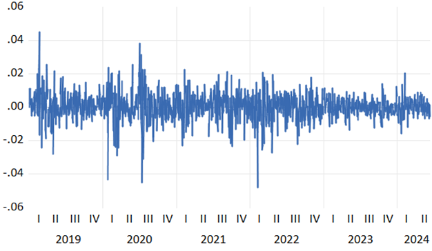
Figure 1: Time series plot of daily returns of the convertible bond index.

The daily return data depicted in Figure 1 exhibits frequent fluctuations around the central axis, indicating significant volatility clustering. Particularly in the mid- term period, there are pronounced fluctuations, suggesting that volatility is not constant but exhibits time-varying characteristics, known as conditional heteroskedasticity. Therefore, to further validate this hypothesis, conducting an ARCH test is deemed necessary.

Augmented Dickey-Fuller Test

Before establishing the ARMA-GARCH model, it is necessary to ensure that the data belong to a stationary time series. Therefore, in this section, the Augmented Dickey- Fuller (ADF) test is employed to verify whether the daily yield of convertible bond index exhibits a unit root. Absence of a unit root indicates that the series is stationary. The regression equation for ADF is as follows:

1 2 1 1 1 Ä Ó Ä p t t i i t Y Y Y t β β δ α ε − = − = + + + + (8) The model’s null hypothesis is: H0:δ=0, H_1:δ<0. If the test results show that the coefficient δ is statistically significant at 0, it indicates that the variable is a unit root process; whereas if δ is statistically significant at a non-zero level, it indicates that the variable is a stable process.

The ADF test results for the daily returns of convertible bond index are presented in Tables 2 and 3.

Variable	z-value	1%	5%	10%	p-value	Stability
Daily Return Rate	-30.9724	-3.96501	-3.41322	-3.12863	0	Stable

Table 2: Unit Root Test of Daily Returns for Convertible Bond Index.

Variable	Coefficient	Std. Error	t-Statistic	Prob.
X(-1)	-0.84249	0.027201	-30.9724	0
C	0.001073	0.000438	2.447694	0.0145

Table 3: Unit Root Test of Daily Returns for Convertible Bond Index.

According to the data presented in Tables 2 and 3, the ADF test statistic for the daily returns of the convertible bond index is -30.972. This value is significantly lower than the critical values at the 1%, 5%, and 10% levels. Additionally, the associated P is close to zero, much smaller than the specified significance level of 0.01. This result strongly rejects the null hypothesis H0:δ=0 at the 1% significance level, indicating no unit root issue and confirming the stability of the time series. Consequently, subsequent model construction can proceed.

ARMA(p, q) Model

In the previous section, it was established that the daily returns sequence of the convertible bond index is stationary. Therefore, an ARMA model can be constructed, but before modeling, it is necessary to determine the order (p, q) of the ARMA model. Typically, the order of the model is determined by analyzing the autocorrelation function (ACF) and partial autocorrelation function (PACF) of the series, as each stochastic process exhibits specific patterns in its ACF and PACF. Figure 2 below displays the correlogram and Q-statistic of the daily returns sequence of the convertible bond index.

Figure 2: Correlogram of the daily returns sequence of the convertible bond index.

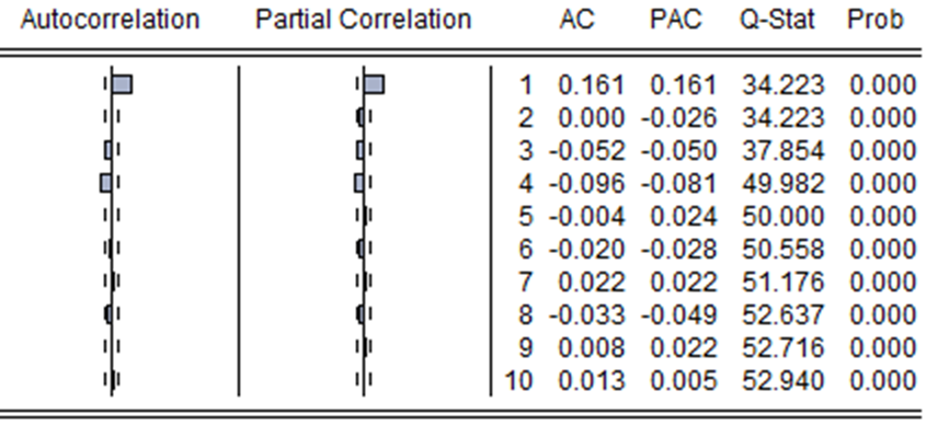
The confidence interval for the autocorrelation coefficients is calculated using the formula 2 2 , n n   −     , n=1322 resulting in a computed interval of (-0.055, 0.055). Analyzing the results in Figure 2, it is found that the time series yt exhibits trailing in both autocorrelation and partial autocorrelation. According to the automatic selection of the best ARIMA lag order in Eviews 12.0 software, it is determined that the model performs best when p is 4 and q is 1, with an AIC value of -6.8380. Therefore, this paper establishes an ARMA(4,1) model. The regression results for the daily returns yt are shown in Table 4.

Variable	Coefficient	Std. Error	t-Statistic	Prob.
AR(4)	-0.08984	0.022428	-4.0058	0.0001
MA(1)	0.162173	0.020035	8.094463	0
SIGMASQ	6.25E-05	1.47E-06	42.63158	0

Table 4: ARMA(4, 1) Model.

Based on the results in Table 4, the final formulation of the ARMA(4, 1) model is as follows:

1 1 0.000063 0.089842 0.162173 t t t t y y ε ε − − = − + + (9)

ARCH Test

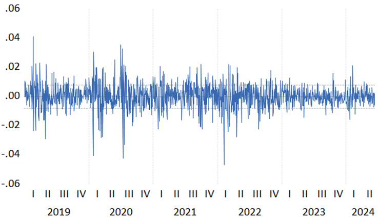
Analyze the time series plot of the residuals obtained from the above regression. As shown in Figure 3 below, significant volatility clustering is evident, suggesting potential conditional heteroscedasticity in the model. Therefore, an ARCH test is needed.

Figure 3: Time Series Plot of Residuals from the Regression Equation.

Since the data used in this paper are daily data with a relatively large sample size, the lag order is chosen to be 10 in the ARCH effect test. The test results are shown in Table 5. The p-values of the F-statistic and LM test statistic are significantly less than 0.01, rejecting the null hypothesis at the 1% significance level. This indicates that the daily returns yt exhibit heteroscedasticity, specifically ARCH effects. Therefore, it is necessary to establish a GARCH model to correct for ARCH effects.

ARCH	Statistical Value	p-value
F-statistic	14.18495	0
Obs*R-squared	128.9854	0

Table 5: ARCH-LM Test.

Garch Model

GARCH(1,1) Model

As previously demonstrated, the time series of daily returns for convertible bonds exhibits ARCH effects. This section will establish a GARCH(1,1) model to correct the aforementioned ARCH model. The correction results are presented in Table 6 below.

Variance Equation
C	1.66E-06	4.78E-07	3.471372	0.0005
RESID(1)^2	0.158949	0.015957	9.960883	0
GARCH(-1)	0.827022	0.018465	44.78909	0
Heteroscedasticity Test: ARCH	0.827022	0.018465	44.78909
F-statistic	0.312572	Prob. F(10, 1297)	0.9782
Obs*R- squared	3.144655	Prob. Chi- Square(10)	0.9778

Table 7: Results of the GARCH(1, 1) Model.

From the results in Table 6, it can be observed that the estimated constant term in the variance equation is 1.66E- 06=0.0000017, which is very small. However, the p-value is 0.0005, significantly less than 0.01, indicating statistical significance at the 1% level. Therefore, the GARCH model established in this section is effective. According to the regression results, the estimated coefficients for the ARCH and GARCH terms are α=0.158949, β=0.827022, respectively. Their sum, α+β=0.985971, is less than 1, complying with the constraints of GARCH model parameters. This suggests that the conditional variance of the error term can converge to the unconditional variance. The formulation of the variance equation is as follows:

2 2 2 1 1 0.0000017 0.158949 0.827022 t t t σ µ σ − − = + + (10)

To further verify the correction of the ARCH effect by the GARCH model, this paper conducted another ARCH effect test with a lag order of 10. The specific test results are shown in Table 7 below.

Heteroskedasticity Test: ARCH
F-statistic	0.341813	Prob. F(10, 1301)	0.9696
Obs*R- squared	3.437999	Prob. Chi- Square(10)	0.9692

Table 6: ARCH-LM Test.

According to the test results in Table 7, the p-value is greater than 0.1, indicating failure to reject the null hypothesis at the significance level, suggesting the absence of conditional heteroscedasticity in the residual sequence. Therefore, the ARCH effects have been successfully corrected, confirming the effectiveness of the model.

Furthermore, the coefficient sum in the GARCH model, α+β=0.984572, is close to 1, indicating that past shocks have a persistent impact on future conditional variance forecasts. This implies that historical convertible bond returns contain information for predicting current returns, and incorporating past risk factors into the model estimation process enhances the forecast accuracy of current volatility. Therefore, constructing the GARCH-M model provides an effective approach to deeply analyze these dynamic effects.

GARCH-M(1,1) Model

To investigate the presence of lagged effects, specifically whether past market factors influence current returns, this study establishes a GARCH-M(1,1) model for further analysis. The results are presented in Table 8 below.

Variance Equation
C	1.50E-06	4.31E-07	3.486612	0.0005
RESID(1)^2	0.140746	0.016481	8.539735	0
GARCH(-1)	0.843826	0.018069	46.69969	0

Table 8: Results of the GARCH-M Model.

According to the test results in Table 8, the estimated constant term in the variance equation is 1.50E- 06=0.0000015, which is very small. However, the p-value is 0.00005, significantly less than 0.01, indicating statistical significance at the 1% level. Therefore, the establishment of the GARCH-M model in this section is effective. Based on the regression results, the estimated coefficients for the ARCH and GARCH terms are α=0.140746 and β=0.843826, respectively. Their sum, α+β=0.984572, is less than 1, adhering to the constraints of GARCH model parameters. This suggests that the conditional variance of the error term can converge to the unconditional variance. The formulation of the variance equation based on the regression results is as follows:

2 2 2 1 1 0.0000015 0.140746 0.843826 t t t σ µ σ − − = + + (11)

To further demonstrate that the GARCH model has corrected the ARCH effect, this paper conducted another ARCH effect test with a lag order of 10. The results are shown in Table 9 below.

According to the test results in Table 9, where P>0.1, the null hypothesis fails to be rejected at the significance level, indicating that the residual sequence no longer exhibits conditional heteroscedasticity. Therefore, the ARCH effects have been successfully corrected.

In summary, the empirical results of the GARCH-M(1,1) model indicate that in China’s convertible bond market, the current volatility of returns is related to past risk factors. Past risk can be utilized to forecast current return volatility. Hence, it can be inferred that China’s convertible bond market has not yet reached weak-form efficiency.

Conclusion

Through the establishment of the ARMA-GARCH model, it was found that the coefficients of the ARCH and GARCH terms are significant at the 1% level. This indicates that past market volatility significantly influences current daily returns of convertible bonds. Furthermore, upon establishing the ARMA-GARCH-M model, similar results were observed with the coefficients of the ARCH and GARCH terms passing the significance test at the 1% level. This suggests that in China’s convertible bond market, the volatility of current returns is closely related to historical risk levels, implying that historical risk data can effectively predict current return volatility. Overall, these model analyses tend to indicate that China’s convertible bond market has not yet met the conditions for weak-form efficient market hypothesis.

To promote the development of China’s convertible bond market towards weak-form efficiency, this paper proposes several recommendations:

Firstly, enhance market transparency. Companies issuing convertible bonds should provide more detailed, timely, and transparent disclosure of information, especially concerning significant events and financial conditions. This can reduce information asymmetry and enhance investor trust in the market. Establishing or improving independent rating agencies to objectively assess convertible bonds will enable investors to better evaluate risks.

Secondly, improve investor education. In China’s convertible bond market, private investors dominate while institutional or professional investors play a secondary role. Private investors often lack theoretical and practical knowledge, and they may have lower risk tolerance and be susceptible to market sentiment, leading to irrational price fluctuations. Addressing these issues requires stricter regulation of information disclosure, attracting and nurturing more institutional investors, and strengthening investor education programs. This aims to introduce more long-term capital, expand market size, and deepen market liquidity.

Thirdly, strengthen regulatory oversight. Rigorously combat insider trading and market manipulation to uphold market fairness and integrity. Develop and refine regulations governing the issuance and trading of convertible bonds to ensure transparency and fairness throughout the issuance and trading processes.

Conflict of Interest

We have no conflict of interests to disclose and the manuscript has been read and approved by all named authors.

References

Fama EF (1965) The Behavior of Stock Market Prices. Journal of Business 38: 34-105.
Andrew WL, Mackinlay AC (1988) Stock Market Price Do Not Follow Random Walks Evidence from a Simple Specification Test. Review of Financial Studies 1(1): 41- 66.
Chen X, Chen X, Bin G (1997) Empirical Study on Weak- form Efficiency of China’s Stock Market. Accounting Research 9: 13-17.
Jiaquan X, Yang Z (2005) Empirical Study on Stock Market Efficiency Based on GARCH Model. Statistics and Information Forum 3: 57-60.
Zan X (2016) Is China’s Stock Market Weak-form Efficient. National Business Review 6: 67-68.
Zhang G, Zhang X (2016) Research on SVM-GARCH Stock Price Prediction Model Based on Nearest Neighbor Mutual Information. Chinese Journal of Management Science 24(9): 11-20.
Yang Q, Xianbing C (2016) Stock Price Analysis and Forecasting Based on ARMA-GARCH Model. Practice and Understanding of Mathematics 46(6): 80-86.
Zhong Q (2017) Stock Price Analysis and Forecasting Based on ARMA-GARCH Model. China Market 1: 68- 69+75.
Shuya X, Liang X (2019) Stock Price Forecasting Research Based on ARIMA-GARCH Model. Journal of Henan Institute of Education 28(4): 20-24.
Wang Y (2021) Analysis and Forecasting of Stock Prices Based on ARMA Model. Productivity Research 9: 124- 127.
Kang H, Ruiyang G (2021) Forecasting Shanghai- Shenzhen 300 Index Prices Based on ARMA Model. Economic Management Abstracts 18: 169-171.
Gan F (2022) Forecasting Study of ChiNext Index Based on ARMA-GARCH-ConvLSTM Hybrid Model. Shenzhen University.
Gaiwen G, Wang S (2023) Stock Price Forecasting Based on Grey Theory and ARIMA Model. Journal of Henan Institute of Education 32(2): 22-27.
Zhang T, Tianxin X (2020) Research on the Efficiency of Offshore RMB Corporate Bond Market: A Comparison Before and After RMB Inclusion in the SDR Basket. Journal of Liaoning University 48(4): 47-58.
Box GP, Jenkins GM (1976) Time series analysis forecasting and control. Journal of Time 31(4): 238-242.
Bollerslev T (1986) Generalized autoregressive conditional heteroskedasticity. Journal of Econometrics 31(3): 307-327.
Robert E (2001) The Use of ARCH/GARCH Models in Applied Econometrics. Journal of Economic Perspective 4: 157-168.

← Previous Article An Empirical Study on the Efficiency of China's Convertible Bond Market Next Article → Very Highly Advanced Artificial Intelligence (VHAAI)