Exploring the Evolution of Quantum Computing: A Comparative Study of Grover’s Algorithm and Conventional Binary Search

Wheeler S¹*, Putta N² and Jakka VR²

¹Clinical Assistant Professor, College of Information, University of North Texas, USA ²College of Information, University of North Texas Denton, Texas, USA

Abbreviations

CPU: Central Processing Unit; QFT: Quantum Fourier Transform; QNNs; Quantum Neural Networks; MRI: Magnetic Resonance Imaging; CT: Computed Tomography.

Introduction

We have seen quite a few technological revolutions taking place since the 20th century, from personal computer production to the internet revolution. Now, we are about to see a similar kind of revolution in computing to Quantum computing. This offers drastically advanced and capable computing systems, where a classical computer might struggle with the load or be unable to process effectively and efficiently.

This literature review aims to explore the historical development of quantum computing back in 1900s, crucial milestones, and important principles of quantum mechanics such as superposition and entanglement. Quantum computers make use of these principles to develop algorithms that outperform classical computers in various tasks. Among the existing algorithms, we decided to focus on the key algorithm Grover’s search algorithm and compare its theoretical performance with a classical binary search. Grover’s algorithm is developed to search unsorted databases with increased speed and high probability of success, whereas for classical search algorithms, these tasks can be very difficult to achieve.

Presently, quantum computing is still in its early stages, where hardware requirements limit practical applications. However, notable progress has been made particularly in the fields of computing power and algorithm development. IBM, a leading business organization, has managed to produce a capacity of 456 qubit quantum machine on IBM cloud. With ever increasing computing power, application of Grover’s algorithm in unsorted database search for large databases is made easy and gives significant speedup compared to classical search algorithms. This makes it an excellent choice for comparison with traditional linear/binary search in terms of performance and time complexity. By comparing the performance of Grover’s algorithm alongside with binary search, the literature review will provide insights into how quantum algorithms might revolutionize data search and retrieval pro-cesses, which are important to large-scale data management in data science. Through this exploration, we expect to deepen our understanding of the principles of quantum algorithms and their potential advantages over classical algorithms in solving complex problems.

History of Quantum Computing

1. Planck and the Black Body Spectrum (1900)

Planck made a breakthrough in 1900 by solving the puzzle of the black body spectrum, which gave a roadmap to future researchers. Planck’s law states that energy of electromagnetic radiation exists in discrete packets or quanta. Then proposed an equation on allowed energies for an electromagnetic radiation with a given frequency. Planck assumed that light behaves as particle and introduced the concept of quantum to explain how energy is transmitted in discrete particles [1].

$$E_n = nhf$$

Where $n$ is a positive integer, $h$ is Planck constant.

2. Einstein and the Photo-Electric Effect (1905)

In 1905, Einstein also proposed that radiation occurred in discrete packets of energy, rather than a continuous form of energy. This led to the idea of photoelectric effect, which states that electrons are emitted from metal when they are exposed to light and introduced the quantized radiation.

From the photo electric effect, Einstein introduced the particle nature of light and played a significant role in proposition of wave-particle duality [2].

$$E_{\text{photon}} = hv - \phi$$

(2)

3. Rutherford’s Discovery of the Atomic Nucleus (1909)

Rutherford conducted the famous gold foil experiment. Alpha particles were fired at thin sheets of gold foil to gain insights on the shape of atoms. The conclusions were drawn from the deflections of rays from gold foil. The amount of deflection at the center has led Rutherford to conclude that a positively charged nucleus is present and surrounded by electrons [2].

4. Bohr’s Model of the Atom (1911)

Bohr after learning about the nucleus, wanted to learn the reason behind the electrons staying in their specific orbits. Bohr proposed that electrons can only occupy specific orbits, and they transition between these orbits by absorbing or emit-ting radiation. Since each orbit has fixed energy, that explains the stability of atoms [2].

5. De Broglie’s Theory of Matter Waves (1924)

De Broglie extended the work about light particles by introducing the concept of matter waves. De Broglie indicated that matter exhibits both wave-like and particle-like properties. Then extended this concept to particles of atoms, such as electrons. De Broglie was able to apply this concept to photons as well and extended the wave-particle duality. Which made the understanding of Planck’s law of Black body radiation significantly easier [1].

6. Heisenberg’s Matrix Mechanics (1925)

Heisenberg used advanced mathematical techniques and proposed matrix mechanics for describing quantum systems [2]. Matrix mechanics states that observables are expressed by matrices. The eigen values of hose matrices can be taken as possible values of observables. And the corresponding eigen vector can be considered as a state of quantum system [1].

7. Schro’Dinger’s Wave Mechanics (1926)

In 1926, Schro’dinger proposed a theory named wave mechanics, it described the state of quantum system using wave function [2].

8. Heisenberg’s Uncertainty Principle (1927)

Heisenberg uncertainty principle has been proved a major contribution in quantum field in late 1920s as a fundamental concept of physics. It states that we cannot estimate the position and momentum simultaneously for a pair of positions. If we try to measure a particle's position with high precision, it leads to uncertainty in measurement as well. The uncertainty principle can be explained using matrix mechanics, if we measure the observable simultaneously, that means the state of quantum system, is same for both indicating same eigen vector. He eigen vectors are not usually same and it can be deduced that we cannot precisely measure observables at the same time [1, 3].

$$\Delta p \Delta x \geq \frac{h}{4\pi}$$

9. Paul Dirac Bra-Ket notation (1930)

Paul Dirac unified quantum mechanics with theory of relativity and proposed a framework for relativistic quantum mechanics. Dirac developed an equation for the electron's behaviour including frequencies spectrum popularly known as Dirac equation. Dirac predicted existence of antiparticles such as positron which was later confirmed experimentally by Carl Anderson in 1932.

Dirac also introduced a mathematical notation for quantum mechanics known as Bra-Ket notation or Dirac notation. This notation is important in quantum mechanics as it simplifies the formalism of quantum mechanics and describes quantum states and transformations.

Bra-Ket is represented in angle brackets and vertical bars where inner product is written as $(a, b)$ in simpler terms, but in Bra-Ket it is as expressed as below:

$$(a, b) = \langle a | b \rangle$$

$$\langle a |$$ is called the bra and $|b|$ is the ket. The bra represents the row vector (the complex conjugate of the ket) and the ket represents the column vector [1].

$$|\psi\rangle = c_1 |\psi_1\rangle + c_2 |\psi_2\rangle$$

Ket vector equation

$$|\psi\rangle = c_1^* |\psi_1\rangle + c_2^* |\psi_2\rangle$$

Bra vector equation

10. Bell's Theorem and Nonlocality (1964)

In 1960's Bell formulated his famous Bell's theorem, which represented mathematical inequality based on local deterministic reality that stated particle properties are influenced by local factors and independent of distant events to solve EPR (Einstein - Podolsky – Rosen) argument. Quantum mechanics prediction has supported the theory of non-locality – the idea that particles can be connected across large distances [2, 4].

$$S = |E(a, b) + E(a', b) + E(a, b') - E(a', b')| \leq 2$$

11. Richard Feynman (1982)

Richard Feynman observed that few quanta mechanical phenomena simulations could not be performed by classical computers and proposed the concept of quantum computer. Computations are more efficient if they are based on quantum mechanical principles. Feynman illustrated the limitations of classical computers in terms of time and probability when per- forming simulation of quantum systems. He also noticed that classical simulations struggle with increasing complexity and demonstrated the lack of classical computers while simulating quantum phenomena [1].

12. David Deutsch (1985)

David Deutsch in 1985 proposed real computational model for quantum computing called quantum computer. He introduced the idea of quantum turning machine from the model of classical turing machine where this machine works under the concepts of quantum computation and has same computational power. Feynman gave the foundation of quantum computation where Deutsch successfully formulated computation model. He also contributed to the theory of quantum gates and introduced the concept of universal quantum gate [1].

13. Peter Shor (1994)

The researchers above stated many cons on classical computing in specific problem solving and simulations, where the classical computing has a limited power and unable to solve the problem. That's where quantum computers were introduced and explained that computationally complex problems can be solved with the help of it. To solve such problems, we require quantum algorithms that can be utilized in that scenario. One such algorithm is introduced by Peter Shor named quantum algorithm for prime factorization, later known as Shor's algorithm.

RSA (Rivest, Shamir, and Adelman) encryption uses difficulty of prime factorization for large numbers to provide security, no classical computer could not solve this in a reasonable time. Shor's algorithm revolutionized this by implementing a method of solving prime factorization in polynomial time on a quantum computer. It clearly displayed the power of quantum computer compared to classical computer and identified that quantum algorithms can also speed up integer multiplication [1].

14. Grover's Algorithm (1996)

Lov Kumar Grover [3] designed an algorithm in 1996 named Grover's algorithm, used to search through an unstructured database. This type of search requires heavy computational resources compared to a sorted and structured database. He then explained the time complexity of a linear search from a classical algorithm as $O(n)$ and the time complexity of Grover’s algorithm as $O(\sqrt{n})$. The performance difference can be observed when the size of the database increases. This algorithm is clearly defined for handling large datasets, and it has a clear advantage in contrast to classical approaches [1].

15. Present day Advancements (2000s - present)

Quantum Computers have developed significantly over the years, A 7 – qubit quantum computer is first developed at Los Almos National Laboratory in the year 2000 [5]. In 2001, Shor’s algorithm has been successfully implemented by IBM and Stanford University [6]. University of Science and Technology of China accomplished five-photon entanglement in the year 2004. On the other hand, Oxford University came up with first pure-state NMR quantum computer [5].

D- Wave systems created first commercial quantum computer in the year 2011 known as D- wave one, with a processor size of 128- qubit [5]. Later in 2013 D- Wave has upgraded their previous version D-Wave One and released D-Wave two with approximately 512 qubit processing power and in 2015, they introduced D-Wave 2X with 2,048 qubits [6].

In 2016, Google has made 9 qubit machines by simulating hydrogen molecule energy. IBM also entered the quantum world by publicly launching IBM quantum experience a cloud platform with 5-qubit processor boosted researching quantum computing and algorithms. In 2017 Google launched Bristle- cone with 72 – qubit chip where Intel released 49-qubit chip called Tangle Lake. IBM released a quantum computer called Q System One, which transformed the practical quantum computing world [5].

Introduction to Binary Search

A binary search also known as half-interval search, logarithmic search or binary chop. A binary search algorithm that finds target value only in a sorted array. It starts searching for a target value in array by splitting the array into two half’s. First the target value is compared with the middle value of the array if the target value matches the middle value then its position in the array is returned if target and middle value are not equal then the search continues in lower half of the array or upper half of the array. If it is less than middle element it continues search in lower half if it is greater than the middle element it continues search in upper half. As this process is repeated until the target is found the algorithm eliminates every half where the target is not found in each iteration [7].

A binary search algorithm an array should be sorted first in an ascending order. Once this constraint is done to find a key value the algorithm may use three variables $l$, $r$ and $m$ which is left, right and middle. The key value is compared with the middle value of the array if it is not equal and then array is divided into two half’s if the key value is found then the index is returned this process until the key value is found in the array [8].

There is an algorithm for searching for the most efficient sorted data is binary search algorithm. In binary search method search is done by splitting the elements into two parts so search is more effective and method is quite efficient as splitting is done in two directions [9].

1. Time complexity in Binary search

As half of the elements are discarded after every iteration it reduces the problem size exponentially. As an example, let’s consider the search space to be an array of size $n$. After the first iteration, the search space becomes $\frac{n}{2}$; after the second it is $\frac{n}{4}$ and so on. After $k$ iterations, the size of the search space becomes $\frac{n}{2^k}$. When the search space is reduced to 1, we understand that the target element is found through binary search, and the time complexity equation is given by

$$\frac{n}{2^k} = 1$$

$$2^k = 1 \implies k = \log_2(n)$$

Therefore the time complexity of binary search is $O(\log n)$. This complexity can be verified using dafny [10].

2. Optimization of Binary search

As stated above time complexity of binary search is $O(\log n)$ the ASH search algorithm finds the target based on same principle as binary search but it splits the array based on position of target it necessarily need not be in the half this improves the time complexity to $O(\log(\log n))$. While binary search is optimal for uniformly distributed data. Whereas ASH search is more convenient with varying distributions of data. This improvement in search technique reduces the number of iterations to find the target element [11].

Continuing with binary search optimization techniques, Quadratic search algorithm. Quadratic search improves efficiency of search by splitting the search space into four parts instead of two. In binary we compare the target element with middle element and decide the search space for next iteration. Whereas in quadratic we compare with elements at ¼, ½, and ¾ in each iteration. This reduces the time complexity to O(log(n/2)).

Binary search works efficiently on uniformly distributed data, Quadratic search speed up the process by splitting the array into more parts and providing faster results. This search is useful for large datasets [12].

3. Application of Binary Searches

Application of binary searches are spread across various fields, from sorting arrays to complex models like noisy binary search. Noisy binary search is used in scenarios with probabilistic errors when comparing. Notable applications include: • Ranking Systems: This can be considered in the sports field, let’s think of a new tennis player. Noisy binary search helps in ranking this new player by comparing performances with existing players performances. • Admission Processes: A system can be used to define some thresholds in choosing a candidate after reviewing their profile for college admission. The system can later evaluate the qualification and assign a decision for the desired target. • Pricing Strategies: Binary search can be used here to optimize the price to reach breakeven sales target. By modeling probability and success for various prices we can identify the highest price point where it reaches a specific volume of sales and maximize profits [13].

Qubits

In classical computing, bits are represented as 0 or 1, and when measured, they result in either 0 or 1. In quantum computing, these are called qubits, or quantum bits, to define quantum states. Qubits are denoted using Dirac notation or bra- ket notation, which is named after physicist Paul Dirac. In his notation, a quantum bit is represented as x for x and y for y [14].

Qubits are the basic units of quantum computing, for building quantum computers. Qubits must meet the following criteria to be feasible:

1. initialization
2. long coherence times
3. universal gate operations
4. efficient state read- out, and
5. Scalability.

Qubits are built using trapped ions, superconducting circuits and photon polarization [15].

Qubits can exist in superposition unlike classical bits, are represented as below equation:

$$ \left| \psi \right\rangle = \alpha \left| 0 \right\rangle + \beta \left| 1 \right\rangle \tag {8} $$ $$ \left| \alpha \right| ^ {2} + \left| \beta \right| ^ {2} = 1. $$ Where α and β are complex numbers, with This superposition allows qubits to display multiple states at once and helps implement quantum parallelism and improve computational power [16].

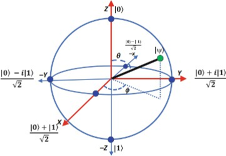
Bloch Sphere Notation of Qubit

The Bloch sphere is a geometric representation of a qubit state in a two-dimensional Hilbert space, where qubits are treated as vectors on the surface of the sphere. For a spin

1

2 −system, it is observed to have two states: spin-up (↑) and spin-down (↓) [17]. It can be written using the linear superposition principle:

$$ \left| \psi \right\rangle = a \left| \uparrow \right\rangle + b \left| \downarrow \right\rangle = \left(\frac {a}{b}\right) $$ (9) Another way to represent the qubit state is using the computational basis, which includes the orthonormal basis:

{ } 0 , 1 [18].

$$ \left| \psi \right\rangle = a \left| 1 \right\rangle + b \left| 2 \right\rangle (1 0) $$ The Bloch sphere is used to represent an individual qubit state. It uses two angles θ and ϕ to map the qubit on the sphere and is expressed as follows:

$$ \left| \psi \right\rangle = \cos \left(\frac {\theta}{2}\right) \left| 0 \right\rangle + e ^ {i \phi} \sin \left(\frac {\theta}{2}\right) \| $$ (11) cos 0 sin 1 2 2 It can also be used to learn qubit manipulation by understanding various rotations of sphere corresponding to qubit operations [16].

Click to enlarge

Quantum Gates

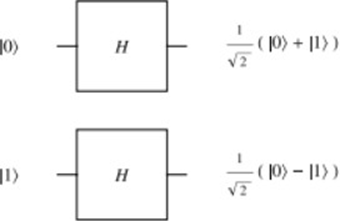
1. Hadamard Gate(H)

The H is gate is one of the important single qubit gates in quantum computing which is represented by the matrix:

$$ H = \frac {1}{\sqrt {2}} \left( \begin{array}{c c} 1 & 1 \\ 1 & - 1 \end{array} \right) $$ (12) The gate connects computational basis states to superposition states and vice versa. For instance, it is given by $$ H | 0 \rangle = \frac {1}{\sqrt {2}} \left(| 0 \rangle + | 1 \rangle\right) \tag {13} $$ $$ H | 1 \rangle = \frac {1}{\sqrt {2}} \left(| 0 \rangle - | 1 \rangle\right) \tag {14} $$ The Hadamard gate produces an equal superposition of all integers ranging from 0 to2 1 n −when it is applied to an n-qubit state, with each qubit initially in the 0 state. This is given by Williams CP [17].

n

2 1 1 0 0 ... 0

$$ \langle \otimes H | 0 \rangle \otimes \dots \otimes H | 0 \rangle = \frac {1}{\sqrt {2 ^ {n}}} \sum_ {j = 0} ^ {2 ^ {n} - 1} | j \rangle \tag {15} $$ n j H H H j

2

0 = Hadamard Transformation on an n-Qubit System

Click to enlarge

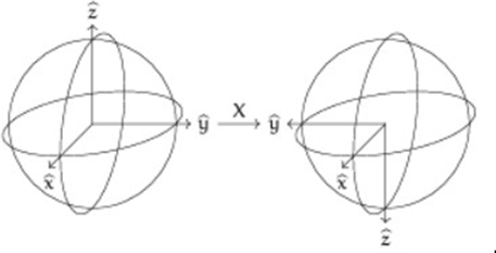
2. Pauli X gate (X)

The Pauli X-gate is one of the fundamental gates in quantum computing and is named after Wolfgang Pauli. It replicates the same function as a classical NOT gate by reversing the state of the qubit [18]. When applied to a qubit, we get the following results:

0 1 →

1 0 → Mathematically, the Pauli X gate can be represented as the matrix below [19]:

0 1 $$ X = \left( \begin{array}{c c} 0 & 1 \\ 1 & 0 \end{array} \right) $$

(16) X gate produces a half-turn of bloch sphere around the x axis [20].

Click to enlarge

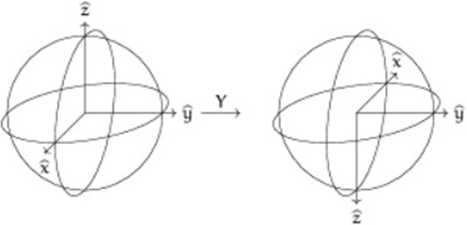
3. Pauli Y gate (Y)

The Pauli Y gate is also considered one of the fundamental single-qubit quantum gates. The matrix form is:

0 i Y i

$$ = \left( \begin{array}{c c} 0 & - i \\ i & 0 \end{array} \right) $$

(17)

0 When the Pauli Y gate is applied, it induces a half-turn (π rotation) around the y-axis of the Bloch sphere. The Y gate can be seen as a combination of the Pauli-X and Pauli-Z gates. In the computational basis, we have:

$$ Y | 0 \rangle = + i | 1 \rangle , Y | 1 \rangle - i | 0 \rangle $$

Thus, the Y gate interchanges 0 and 1 states while also applying a relative phase flip [20].

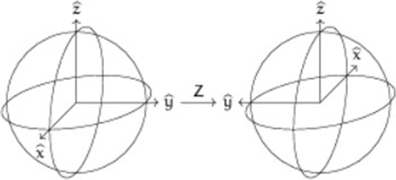
4. Pauli Z gate (Z)

The Pauli Z gate acts in a similar way to the X and Y gates. The Z gate rotates the qubit by π radians around the Z-axis.

When the Z gate is applied to a qubit, 0 is left unchanged, and 1 is mapped to 1 − . The computation matrix for the corresponding output is [21]:

$$ Z = \left( \begin{array}{c c} 1 & 0 \\ 0 & - 1 \end{array} \right) $$

(18) $$ Z \left| 0 \right\rangle = \left| 0 \right\rangle , Z \left| 1 \right\rangle = \left| - 1 \right\rangle $$

Click to enlarge

Click to enlarge

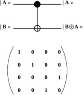
5. CNOT gate

The controlled NOT (CNOT) gate can be compared to the classical XOR gate. It mainly functions on two qubits: a control qubit and a target qubit. When applied to two qubits, the CNOT gate does not change the target qubit if the control qubit is in the 0 state. If the control qubit is in the 1 state, the CNOT gate changes the target qubit by flipping it. Below are the resulting transformations when the CNOT gate is applied to two qubits:

• |00⟩ → |00⟩
• |01⟩ → |01⟩
• |10⟩ → |11⟩
• |11⟩ → |10⟩ Mathematically, the CNOT gate can be represented as , , A B A B A → ⊗ (19) where B ⊕ A is the XOR operation [22].

Quantum Computer Architecture

Architecture of quantum computer varies from the traditional systems, as traditional systems use bits as basic units and utilize Boolean algebra to process data. These computers follow Von Neumann architecture model: which consists of following components: Input/output mechanisms, Central Processing Unit (CPU), and memory systems.

Compared with quantum computers, qubits are used as information units, which can exist in various states at once

Click to enlarge

Processing multiple possible scenarios and leading to a solution. The advantage here is that they rely on principles of superposition and entanglement allowing quantum computers to find solutions more quickly than classical systems [23].

The architecture of a quantum computer focuses on developing systems that work on the principles of quantum computing and quantum mechanics. This is designed to achieve a system that is far better than the existing system in terms of both computing power and capabilities. There are several base components on which a quantum computer can be built: Quantum Arithmetic: Every quantum computer architecture includes quantum arithmetic, involving complex operations such as entanglement and superposition in the development of the machine.

• Cluster-State: This heavily relies on entangled qubits and is structured in a way that allows for improved error tolerance. These systems are designed to reduce errors through error-correcting codes.

• Layered Architecture: In this approach, the processing tasks of a quantum computer are broken down into layers, each with specific roles (such as qubit management and error correction). This system allows each layer to operate semi-independently, making the overall system resilient to errors [24].

**Introduction to Quantum Search Algorithms**

Quantum search algorithms use the principles of quantum computing to perform tasks. One such algorithm is Grover’s algorithm, which is used to address problems in unstructured data search, such as finding a specific element in an unsorted dataset. Usually, it takes $O(N)$ time in classical computing, but Grover’s algorithm achieves a quadratic speedup and reduces the time complexity to $O(\sqrt{N})$.

Quantum search algorithms solve problems which are challenging for classical algorithms. They use principles like quantum superposition, entanglement, and interference to evaluate multiple states within quantum system.

Grover’s algorithm is a probabilistic quantum algorithm, and it amplifies probability of correct solution after every thorough search. This is carried out with the help of quantum oracle and amplitude amplification technique [25, 26].

**Grover’s Algorithm Mechanics**

Grover’s algorithm provides a solution to searching problems in an unordered database. It performs this search in $O(\sqrt{N})$, offering a quadratic speedup.

1. Steps

Initialization: The algorithm begins by registering $n$ qubits, each initialized to the state 0. A Hadamard gate is then applied to each qubit, placing them in superposition across all 2n states. Initially, all states have equal probability amplitude.

$$|\psi\rangle = \frac{1}{\sqrt{2^n}} \sum_{x=0}^{2^n} |x\rangle$$ (20)

Phase Inversion: In this step, the quantum oracle marks the correct state by inverting its phase. This is achieved by multiplying the amplitude by 1, thereby indicating the correct state without changing the probability, only the amplitude.

$$O|\psi\rangle = |-1\rangle^{f(x)} |x\rangle$$ (21)

Diffusion Operator: After the phase inversion, the diffusion operator is applied. This step amplifies the amplitude of the correct state while reducing the amplitude of all other states.

$$D = 2|\psi\rangle\langle\psi| - I$$ (22)

Repetition: The phase inversion and diffusion operator steps are repeated for $O(\sqrt{N})$ iterations. This repetition significantly amplifies the amplitude of the correct state, distinguishing it from the others.

Measurement: After sufficient iterations, the system is measured. The correct state should now have a probability close to 1, making it identifiable.

2. Example Application of Grover’s Algorithm

Consider a qubit size of 3, yielding a search space of $N = 8$.

Initialization: Applying the Hadamard gate to 3 qubits (each representing either 0 or 1) and placing them in superposition gives:

$$|\psi\rangle = \frac{1}{\sqrt{8}} |000\rangle + |001\rangle + |010\rangle + |100\rangle$$ (23)

$$+ |100\rangle + |101\rangle + |110\rangle + |111\rangle$$

This results in an amplitude of $\frac{1}{\sqrt{8}} = 0.354$ for each state.

Oracle Application: Suppose we are searching for $|011\rangle$. The oracle marks this state by applying phase inversion, resulting in:

$$|\psi\rangle = \frac{1}{\sqrt{8}} |000\rangle + |001\rangle + |010\rangle - |100\rangle$$ (24)

$$+ |100\rangle + |101\rangle + |110\rangle + |111\rangle$$

Diffusion Operator: Before applying the diffusion operator, each amplitude is 0.354. After applying the operator, the amplitude of the correct state increases while those of the others decrease.

Iterations: As discussed, $O(\sqrt{N})$ iterations are required. For $N = 8$, we perform approximately 2 iterations. After 2 iterations, the amplitude of the correct state $|011\rangle$ becomes significantly amplified, allowing us to identify it as the solution [27].

**Limitations of Grover’s Algorithm**

Even though Grover’s algorithm provides quadratic speedup in theory, it is practically challenging to build a quantum computer that supports this theoretical proposition [26, 28].

Quantum noise and hardware limitations result in unreliable results on current quantum computers [29].

**Introduction to Quantum Principles**

Superposition: Superposition is a fundamental principle in quantum computing that demonstrates how a qubit can exist in a combination of both 0 and 1 state simultaneously. It can be expressed as

$$\left| \psi \right\rangle = \alpha \left| 0 \right\rangle + \beta \left| 1 \right\rangle$$

$$\left| \alpha \right|^2 + \left| \beta \right|^2 = 1$$

The above condition (26) is used to identify whether a qubit exists in that state or not. This property allows quantum computers to process multiple possible states simultaneously, thereby enhancing the performance of quantum computing.

Entanglement: Entanglement is a phenomenon where multiple qubits become correlated, and the state of one qubit influences the states of other qubits, regardless of the distance between them. Measuring one qubit determines the state of the other qubit instantaneously [23].

Quantum Error Correction: Quantum error correction is an important principle for safeguarding quantum information from noise and unnecessary interference. This type of disturbance in quantum computing is called decoherence. The principle involves encoding states that detect and correct errors without disturbing the information. This is implemented by storing information about errors in a subspace of a larger Hilbert space and moving the quantum state to an orthogonal error space [30].

**Eigen Values and Eigen Vectors**

Eigenvectors are defined for a matrix where it states that when the matrix is transformed using the vector, it only stretches or scales the matrix and does not change the direction. The scalar by which the vector is stretched is called eigen value [31].

This concept plays an important role in quantum computing as a quantum state can be denoted in Hilbert space with the help of this vector and can be treated as eigen value problems. The eigen values here represent quantities such as energy levels and corresponding eigen vectors displays possible quantum states.

$$A v = \lambda v$$

(Eigen value equation for linear transformation $A$, where $\nu$ is the eigenvector and $\lambda$ is the corresponding eigenvalue. It implies that applying matrix $A$ to vector $\nu$, it stretches or compresses the vector by $\lambda$ but does not change the direction [32]).

**Qiskit**

Qiskit, abbreviated as Quantum Information Software Kit, is an open-source SDK (software development kit) for quantum computations on classical machines, developed by IBM [33]. Qiskit enables the design and execution of quantum algorithms on quantum hardware, assisting researchers in building and optimizing circuits for various needs and executing them across multiple available back ends.

One of the strengths of Qiskit is that it allows users to program at various levels, from circuit construction to hardware-specific pulse control, making it a versatile tool for advancing quantum research [34]. Other components of Qiskit extend its capabilities, serving as interfaces and providing additional functionality to enhance the Qiskit workflow. These projects, largely contributed by the open-source community and partly managed by IBM Quantum teams, include IBM Quantum [34].

Qiskit Aer: Qiskit Aer provides an interface for running quantum circuits with or without noise by implementing various simulation methods. This flexibility enables researchers to test and benchmark quantum circuits under different noise models, advancing the development and optimization of quantum Algorithms [28].

Qiskit Machine Learning: Qiskit Machine learning is a robust toolkit that integrates quantum computing with machine learning tasks. It includes components such as Quantum Kernels and Quantum Neural Networks, which can be utilized for diverse applications, including classification and regression. This toolkit introduces a new approach to machine learning that leverages the unique properties of quantum computing [35].

**Quantum Probability Density Function**

The quantum probability density function method describes the rise of quantum probability density functions in space and time. It is constructed with the help of wave function and its complex conjugate.

$$P = \psi^* \psi$$

(28)

Probability based approach is used to describe quantum systems and works well with wave function formalism. Utilizing Schrodinger equation these wave functions also evolve and in this approach the probability density is deduced directly from probabilities. This approach is mainly used in applications like quantum communication and quantum computing. QPDF approach ensures that probabilities are always positive and provides a better and consistent density function for quantum systems [36].

**Quantum Fourier Transform**

Quantum Fourier Transform is an important algorithm that functions like the classical Fourier transform but supported by the power of quantum parallelism exponentially for faster computation. Discrete Fourier transform makes a connection between time and frequency domains for vectors, QFT relates this transformation to quantum states, switches them to superposition of computational basis states. QFT changes a superposition of quantum states $|\phi\rangle$ represented by vectors $|i\rangle$ into Fourier basis on the following equation [37].

$$\psi_k = \frac{1}{\sqrt{N}} \sum_{i=0}^{N-1} \phi e^{\frac{2\pi i k}{n}} |k\rangle$$ (29)

**Applications Of Quantum Computing**

Quantum computing allows major speedups over classical techniques in certain applications, particularly in unstructured search problems.

1. Applications in Search and Optimization

- Searching for a target in unstructured data: Grover’s algorithm provides a quadratic speedup with a time complexity of $O(\sqrt{N})$. It can also be used as a subroutine with amplitude amplification to increase the efficiency of various computational tasks. Some examples include:

1. Finding the Minimum of an Unordered List: In an unordered list of $N$ elements, Grover’s algorithm can find the minimum with $O(\sqrt{N})$ evaluations, while classical computing takes $O(N)$.
2. Graph Connectivity: In large-scale graph analysis, the classical approach takes $O(N^2)$ to determine graph connectivity. In quantum computing, it takes $O(N^{3/2})$, where $N$ is the number of vertices.
3. Pattern Matching: In text processing and bioinformatics, classical pattern matching takes $O(n+m)$ in a text of length $n$ with pattern length $m$.

In quantum computing, it is reduced to $O(\sqrt{n+m})$, which is highly effective for large datasets [38].

2. Applications in Data Science

- Quantum Neural Networks (QNNs): QNNs handle complex computations faster and more accurately in deep learning applications using qubits by utilizing superposition and entanglement principles. They are an extended version of classical neural networks [39].

- Quantum Clustering: For identifying optimal groupings, quantum clustering estimates various clustering possibilities at once, speeding up the process.

- Quantum Dimensionality Reduction: Using techniques of quantum principal component analysis, quantum computing finds principal components in large datasets, simplifying models [40].

3. Applications in Healthcare

- Drug Discovery: Quantum computing allows researchers to simulate molecular interactions to estimate drug efficacy and toxicity precisely. It can also optimize existing drug compounds to reduce costs.

- Precision Medicine: Quantum computing is used to analyze large amounts of data specific to patient genetics and medical information, improving personalized treatment plans.

- Medical Imaging: Quantum computing can improve image quality and reduce noise in scans like MRI and CT. It uses superposition and entanglement to produce accurate, clear images, aiding in early disease detection [41].

4. Applications in Banking and Finance

- Credit Scoring: Quantum computing improves credit scoring techniques by analyzing borrower data from multiple sources rapidly, allowing for accurate scoring and risk assessment, thus optimizing credit allocation.

- Portfolio Management: Identifying an optimal asset mix for a risk-adjusted portfolio is challenging with traditional methods due to an exponential solution space. Quantum computing can evaluate complex combinations and find an appropriate solution in fewer steps [42].

5. Applications in Logistics

- Route Optimization: Quantum computing helps delivery companies find optimized routes by swiftly exploring all available options and identifying the best solution.

- Fleet Management: Quantum optimization algorithms assist in fleet management by effectively deploying vehicles and machines [43].

**Comparison between Grover’s Search Algorithm and Classical Search Algorithms (Peer Review)**

For this peer review we are considering several articles which focused on comparing Grover’s and classical search algorithms to get a proper understanding of methods, relevance, and limitations due to computational challenges. The article by Castillo et al., provided a comprehensive look at Grover’s algorithm, clearly explaining the use of superposition principle to get a quadratic speedup in search tasks. Log N searches for required for binary search algorithm and to perform the same task using Grover’s algorithm takes around (O(sqrtN) steps. This has been achievable using Grover’s algorithm but not by any classical algorithms is because of the mechanism of quantum parallelism which allows searching simultaneously and reflects unique amplitude that increases with each iteration [44].

The extensive article by Kevin also illustrated about the time complexity and iteration count for Grover’s algorithm and covered the probabilistic theory behind Grover’s algorithm. The author also talked about how accuracy is increasing with iterations, displaying speedup compared to classical algorithm. The article covered the usage of both IBM’s Q Experience and Microsoft’s Q# for performing Grover’s algorithm on real- world problems and concluded results when compared to the same task with classical algorithms. The authors observed that with IBM’s quantum simulations, the successful retrieval probability ranged from 75.7% to 90.1%, highlighting limitations in hardware and instability in the quantum system. In contrast, in Microsoft’s Q#, criteria such as the number of amplitude amplifications and marked elements clearly demonstrated their significance in achieving higher success rates through iterations.

This peer-reviewed analysis concludes that Grover’s algorithm has a lot of potential going further once the hardware can accommodate and stabilize all the computational power. Theoretically we can see that there is an exponential improvement and can be proved after building stabilized equipment [45].

This paper has included a brief comparison of grover’s algorithm along with binary search, and sequential search. The authors started by initializing the qubits and their probabilities to 0, and then applied phase inversion to modify amplitude of target state, and at last mean inversion to clearly show amplitude difference of target state with other state. This application of code shows clear how grover’s algorithm reduces error and increases probability in finding target state. From the above experiment, Grover’s algorithm achieved 95% improvement in response time over classical methods [46].

Pseudo Code

1. Function BINARYSEARCH(array, target) 2. Initialize left ← 0

3. Initialize right ← length of array -1 4. Record start time 5. While left ≤ right do 6. Calculate mid ← left + (right - left)//2 7. If array[mid] = target 8. Record end_time 9. Return end_time – start_time 10. Else if array[mid] < target 11. Set left ← mid + 1 12. Else 13. Set right← mid - 1 14. Record end_time 15. Return end_time - start_time (target not found) 16. Function GROVERSEARCH(random dataset, target) 17. Determine n_qubits as the ceiling of log2 of dataset 18. Find oracle_index and convert to binary (oracle bi 19. Define Oracle: 20. For each bit in oracle_binary, apply X gate if t is ’0’ 21. Apply controlled Z gate (cz) 22. For each bit in oracle_binary, apply X gate if t is ’0’ 23. Define Diffusion Operator: 24. Apply Hadamard gates to all qubits 25. Apply X gates to all qubits 26. Apply Hadamard to the last qubit 27. Apply Multi-Controlled X (MCX) gate 28. Apply Hadamard to the last qubit 29. Apply X gates to all qubits 30. Apply Hadamard gates to all qubits 31. Create Grover Circuit: 32. Initialize a quantum circuit with n_qubits 33. Apply Hadamard gates to all qubits 34. Determine grover_iterations, as approximate square root of dataset size 35. For each iteration in grover_iterations, append Oracle and Diffusion Operator 36. Measure qubits 37. Run Simulation: 38. Transpile and execute the circuit 39. Record runtime 40. Return runtime 41. Main Procedure 42. Initialize datasets and target 43. For each of 10 test cases: 44. Run BINARYSEARCH and record runtime 45. Shuffle dataset, ensure target is present 46. Run GROVERSEARCH and record runtime 47. Plot runtime results for Binary Search and Grover’s Algorithm

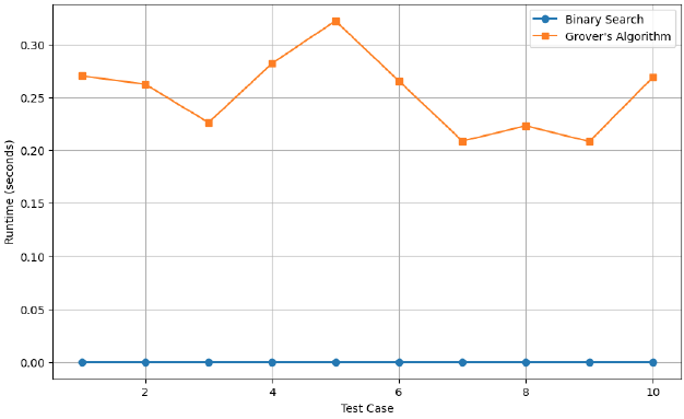
Results

Conducted experiment using 10 random test cases with unique target values for each individual test case. The targets used for the experiments are:

• Target values: 8707, 4644, 2067, 9996, 5298, 7523, 8837, 5906, 734, 991 • The average runtime for each algorithm across all test cases is: • Binary Search: Average Runtime: 0.000000 seconds • Grover’s Algorithm: Average Runtime: 0.253801 seconds

Click to enlarge

Hypothesis

In this study, we hypothesize that Grover’s algorithm will give a lower response time on unsorted dataset compared to binary search on sorted dataset. Grover’s algorithm requires fewer iterations than binary search with increasing size of dataset.

Null Hypothesis

The null hypothesis for this study is that binary search algorithm is executed quickly and has lower response time compared to Grover’s algorithm on a unsorted dataset.

Conclusion

The computational comparison results of Binary Search and Grover’s Algorithm did not align with the original hypothesis. From the statistical analysis, it was observed that the p-value is greater than the significance level (α = 0.05), indicating that there is insufficient evidence to reject the null hypothesis. Consequently, we reject the alternate hypothesis and conclude that the data observations do not support the claim that Grover’s Algorithm is faster than Binary Search.

The contributing factors in achieving the above results: The computation is done using Qiskit a quantum simulation platform where it is a 5-qubit simulator running on the classical computer, which significantly differs from the performance of a real quantum computer. Qiskit is used widely by numerous researchers and developers simultaneously which can lead to computational overload and reduce the performance during simulation. Overhead of simulation and size of dataset might have prevented Grover’s algorithm from outperforming Binary search.

In this study, we examined the response time as performance metric for Grover’s algorithm compared to classical search algorithms (binary search). Our initial hypothesis suggested that Grover’s algorithm would demonstrate a quantum speedup, leading to significantly lower response times. However, the experimental results did not align with this hypothesis. Instead, our findings indicate that Grover’s algorithm does not provide a significant advantage in response time over binary search in this specific experimental setup. The data thus supports the null hypothesis, which posits that there is no measurable difference in performance between the two algorithms under the conditions tested. The source code for this analysis which contains implementation of Binary Search and Grover’s Algorithm and runtime comparisons, is available in GitHub repository [47].

Going forward testing the Grover’s algorithm on a real quantum computer should be the main focus to overcome the limitations of simulations and clearly validate the quadratic speedup in a practical scenario. That would set a foundation for Grover’s search algorithm on large unsorted datasets. With the increasing size of data collected, processed on a daily basis, incorporating quantum computing into data science workflows help breakthroughs in fields of machine learning and optimization, and data analytics.