Sonic Log Simulations in Wells of Campos and Santos Basins
The well log is one of the main tools in the oil fields exploration, as it allows an interpretation of the petrophysical characteristics and provides reliable calculations of the volume of oil and water contained in the reservoir. The basic logs are gamma rays (GR), resistivity (RT), density (RHOB), neutron (NPHI) and sonic (DT). The sonic log is used for porosity calculations, fracture identification and seismic attributes inversion, providing important estimates of the physical properties of perforated rocks. Despite this importance, often the sonic log is not available, due to data loss in old wells, technical failures during its acquisition or by economic necessity. In this case, the nonexistent log is obtained through synthetic models that associate other basic logs with the sonic log. One of the most used models was developed by Gardner et al. (1974), who relates the velocity of the compressional wave (VP) to the density but does not always obtain satisfactory results. As an alternative, several investigators applied methods such as Neural Network, Fuzzy Logic and Multiple Linear Regression, correlating VP with other well logs, besides density. The objective of this work was to compare the results of the Multiple Linear Regression (MLR), Neural Network (NN), Fuzzy Logic (FL), Geological Differential Method (GDM) and Gardner model of simulation of the sonic log (VP), from well logs of 57 wells located in the Campos and Santos Basins, with presence of siliciclastic and carbonatic rocks of the post and pre-salt. The results obtained showed that the techniques are efficient, except the Fuzzy Logic and Neural Network. The Gardner model proved to be efficient even using only the density log to simulate VP, but in regions with higher porosity presented inferior results to the MLR and GDM techniques, which used the resistivity and gamma ray logs, besides density, representing better the effects of the fluids on the sonic log
Introduction
Well logging is one of the most important tools in the oil fields exploration, because it allows a petrophysical characteristics interpretation and provides reliable calculations of the volume of oil and water contained in the reservoir. The basic logs used are gamma rays (RG), resistivity (RT), density (RHOB), neutron (NPHI) and sonic (DT) [1, 2].
The sonic log has a great contribution to the well- seismic tie, seismic interpretation, lithological identification, determination of geopressions, identification of fractures and inversion of seismic attributes, providing important estimates of the physical properties of perforated rocks. However, this log is not available in many wells, either due to data loss in old wells, failure during acquisition or cost reduction [3]. Usually, this problem is solved by simulating the log from other available data, such as using rock physics models, petrophysical properties of plugs and data from other well logs, such as density and resistivity, but the results are not always satisfactory [4].
An important model for predicting the sonic log from other well logs was developed by Gardner, et al. [5], where the density log is correlated with the P-wave velocity log ($V_p$). This model is an alternative to model developed by Faust [6], which correlates P-wave velocity log ($V_p$) with resistivity log.
Currently, many studies have used recent mathematical methods to predict the sonic log, among them Multiple Linear Regression (MLR), Fuzzy Logic (FL) and Neural Networks (NN) [1, 4, 7, 8, 9, 10, 11]. A characteristic observed in these studies is the use of data from few wells and rocks of low complexity, limited to regions that characterize a reservoir. In a different way, our work applied several mathematical techniques, in addition to the geological differential method (GDM), in a larger number of wells, in carbonate reservoirs of the post and pre-salt of the Brazilian Basins of Campos and Santos. In addition, the entire length of the well logs was taken advantage of, which is a common situation faced in the oil industry.
**Materials and Methods**
For this work, 133 wells from 6 different oil fields were made available, including 4 post-salt fields in the Campos Basin (130 wells) and 2 pre-salt fields in the Santos Basin (3 wells). These data were loaded in the software Interactive Petrophysics [12] and the basic suit of logs (density, resistivity, gamma and sonic) were plotted. Then, the wells containing the logs in good condition were selected, resulting in a set of 57 wells, including 3 pre-salt wells and 54 post-salt wells. Part of the data is public, which is the case of the Namorado field, located in the Campos Basin, while the other data were provided by Petrobras and Petrogal. Figure 1 presents a schematic of the data available and used at this work.
Looking for an improvement of the $V_p$ simulations, markers were created separating the regions of the wells with predominance of siliciclastic rocks and another one with carbonate rocks. Of the 57 wells, 51 have intervals with predominance of siliciclastic rocks and 48 wells have intervals with predominance of carbonate rocks.
**Gardner Model**
The Gardner, et al. [5] model was applied to all 57 wells using Equation 1.
$$V_p = \left( \frac{\rho_b}{a} \right)^{\frac{1}{b}}$$
where $V_p$ is the P-wave velocity in km/s, $\rho_b$ the density in gr/cm$^3$ and, the terms $a$ and $b$ are adjustment coefficients, whose values are 0.23 and 0.25, respectively.
For the remaining methods (MLR, FL, NN and GDM), only the 54 post-salt wells were used to construct the models, whereas the 3 pre-salt wells were used as a blind test. Unlike the Gardner model, which uses only the density, these methods predicted the sonic log from the density, resistivity and gamma ray logs. In addition, the simulations were performed using modules available in Interactive Petrophysics software.
**Multiple Linear Regression (MLR)**
MLR is the study of how a dependent variable $y$ is related to two or more independent variables $x$, where in this case the dependent variable is the compressional velocity log and the independent variables are the density, resistivity and gamma ray logs. It is described according to Equation 2.
$$y = \beta_0 + \beta_1 X_1 + \beta_2 X_2 + \dots + \beta_p X_p + \varepsilon$$
The terms $\beta_a, \beta_b, \beta_c, \dots, \beta_p$ are the parameters and the term $\varepsilon$ (error) is a random variable. Analyzing this model, we observed that $y$ is a linear function of $x_1, x_2, \dots, x_p$ plus the error term $\varepsilon$. The error term is responsible for the variability in $y$ which cannot be explained by the linear effect of the independent $p$ variables.
In this work two models were constructed, for the first model, called the general model, the 54 post-salt wells and the entire length of the logs were used. The second model, called the lithological model, was constructed considering previously separated areas of siliciclastic and carbonate rocks. With this, the curves VP_MLR (general model) and VP_MLR_LITO (lithological model) are generated [13].
**Fuzzy Logic (FL)**
In the FL used in this work, the training data are classified in almost equal compartments, beginning with the lowest values, and extending to the highest ones. For the data set, the mean ($\mu$) and the standard deviation ($\sigma$) are calculated for all associated curves used for the prediction. Then the mean and standard deviation values are used to find the most likely outcome in the prediction [9]. To make the prediction, the fuzzy probability that an input log is in each set is first calculated using Equation (3).
$$P(C_b) = \sqrt{n_b} X e^{-(c - \mu_b)^2 / (2X\sigma_b^2)}$$
The terms $P(C_b)$ is the probability that the curve $C$ is in the set $b$, $n_b$ is the number of samples in set $b$, $C$ is the input value for curve $C$, $\mu$ is the mean of the curve $C$ for the set $b$ and $\sigma_b$ is the standard deviation of curve $C$ for set $b$. The probabilities of all input curves are then combined from Equation (4).
$$\frac{1}{P_b} = \frac{1}{P(C1_b)} + \frac{1}{P(C2_b)} + \frac{1}{P(C3_b)} + \dots$$
The term $P_b$ is the total probability for the set $b$ and $P(C1_b)$ is the probability of the curve $C1$ for the set $b$. The solution will be the set most likely (LR Senergy) [12].
During the prediction process, the number of sets was changed manually to find the best result and the value found was equal to 2. The model was constructed using the lithological separation mentioned above and resulted in the VP_Fuzzy curve.
**Neural Network (NN)**
In the Neural Network the data are received by the neurons in the input layer and transferred to the neurons in the first hidden layer through the weighted connections. These data are processed mathematically and transferred to the neurons in the next layer. The output of the network is provided by the neurons in the last layer. The j-th neuron in a hidden layer processes the received data $(x_i)$ by: (i) calculating the weighted sum and adding a “polarization” term $(\theta_j)$ according to Equation (5) [14].
$$net_j = \sum_{i=1}^{n} x_i \times w_{ij} + \theta_j j = (1,2,3,n)$$
The model was also constructed using the lithological separation and resulted in the VP_Neural curve.
**Geological Differential Method (GDM)**
The GDM technique is designed to use all the positive features of commonly applied statistical methods (MLR, Fuzzy Logic, Genetic Algorithms, Neural Network), but instead of using them to provide a basis for inference, use them as part of a predictive process. It was developed in works that aimed at the prediction of logs from data obtained from the measurement of gas in the drilling fluid.
The technique is based on the inclusion and extraction of the maximum value of all input data, optimizing the value of all available data and producing a point-to-point solution through the method of finite differences with high number of iterations [15, 16, 17].
As with the MLR method, two models were constructed: a general model that resulted in the VP_GDM curve and another considering the lithological separation, resulting in the curve VP_GDM_Lito.
**Goodness of Fit**
After fitting data with one or more models or estimates, you should evaluate the goodness of fit and, for that, some metrics are used. They show trends of increasing or decreasing values, relative to the previous value of the same metric. Thus, after obtaining the simulated curves, the data were exported to the Microsoft Excel software, where the Root Mean Square Error (RMSE) and the Pearson correlation (R) and determination ($R^2$) coefficients were calculated. Thus, the Root-Mean-Square Error (RMSE) is a frequently used measure of the differences between values predicted by a model or an estimator and the values observed. It is calculated by the square root of the second sample moment of the differences between predicted values and observed values or the quadratic mean of these differences. These deviations are called residuals. $R$, on the other hand, is a measure of linear correlation between two sets of data. It is the covariance of two variables, divided by the product of their standard deviations. Finally, $R^2$ (R squared), is the proportion of the variance in the dependent variable that is predictable from the independent variable(s). It provides a measure of how well observed outcomes are replicated by the model. In summary, RMSE is the quantification of the adjustment error, R provides na idea of the variance of the estimate and, $R^2$ gives a notion of how much the estimate resembles the data [18].
**Applications & Results**
**Post-Salt Wells**
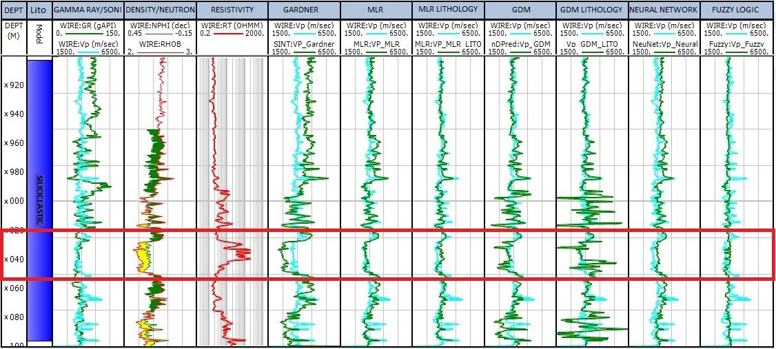
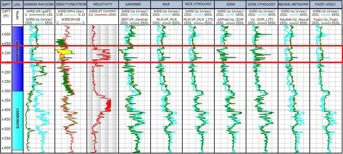
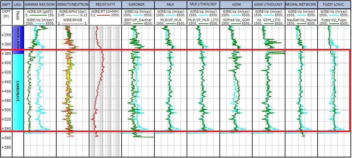
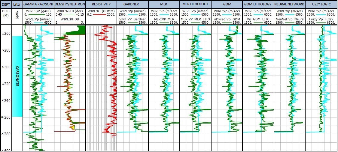
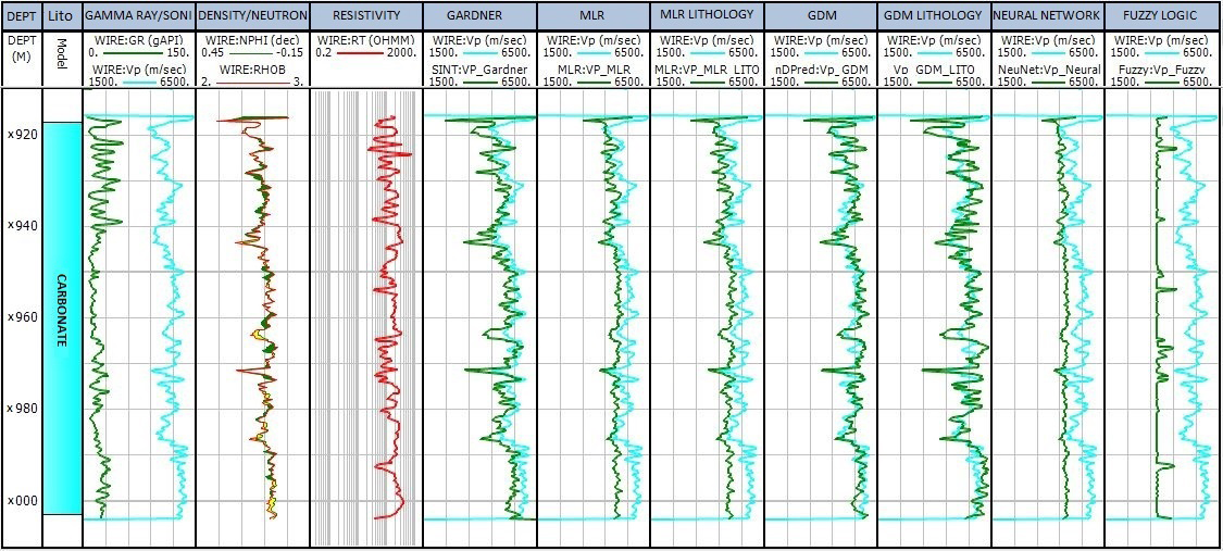
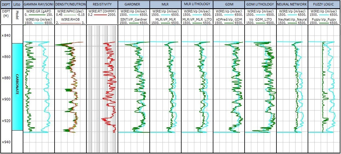
The simulated curves of the compressional wave velocity and the basic suite of logs (gamma rays, resistivity, density and VP) of 3 post-salt wells are presented in Figures 2-4, highlighting some situations where errors occurred in the simulations.
The figures are plotted from left to right, the tracks with the well depth, the lithologic classification (siliciclastic and carbonate rocks), basic logs gamma ray (green) and P
velocity (blue), density (red) and neutron (green), resistivity (red). The following tracks present the Vp log (blue) with simulated curves, in order: Gardner model, Multiple Linear Regression (general model), Multiple Linear Regression (lithological considerations model), Geological Differential Method (general model), Geological Differential Method lithological considerations), Neural Networks and Fuzzy Logic. In all these figures, the depth appears written with an “x” in front of the numbers, in order to hide the true depth, due to the need to observe the confidentiality of the data.
Analyzing Figures 2 through 4, it can be observed that the simulated logs from Neural Networks (Vp_Neural) and Fuzzy Logic (Vp_Fuzzy) generated curves with low variation, presenting little representativeness to the geological variations, although they approach the Vp log. The simulated logs by MLR and GDM presented good results, which diverged from the original curve at small depth intervals and were slightly better than Gardner.
Comparing the Gardner curve with the others, it is observed that this diverges from the original curve mainly in reservoir regions. This is because that the higher porosity and consequently the greater amount of fluid causes in the density and sonic logs. As the model in question is a direct relation between the velocity of the P wave and the density, this effect causes a distortion in the simulated curve, whereas in the other methods this effect is reduced due to the use of the resistivity log. Similarly, small distortions in regions with shale presence were mitigated using the gamma ray log in the other methods.
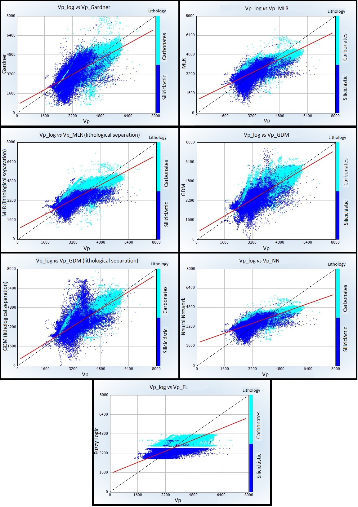
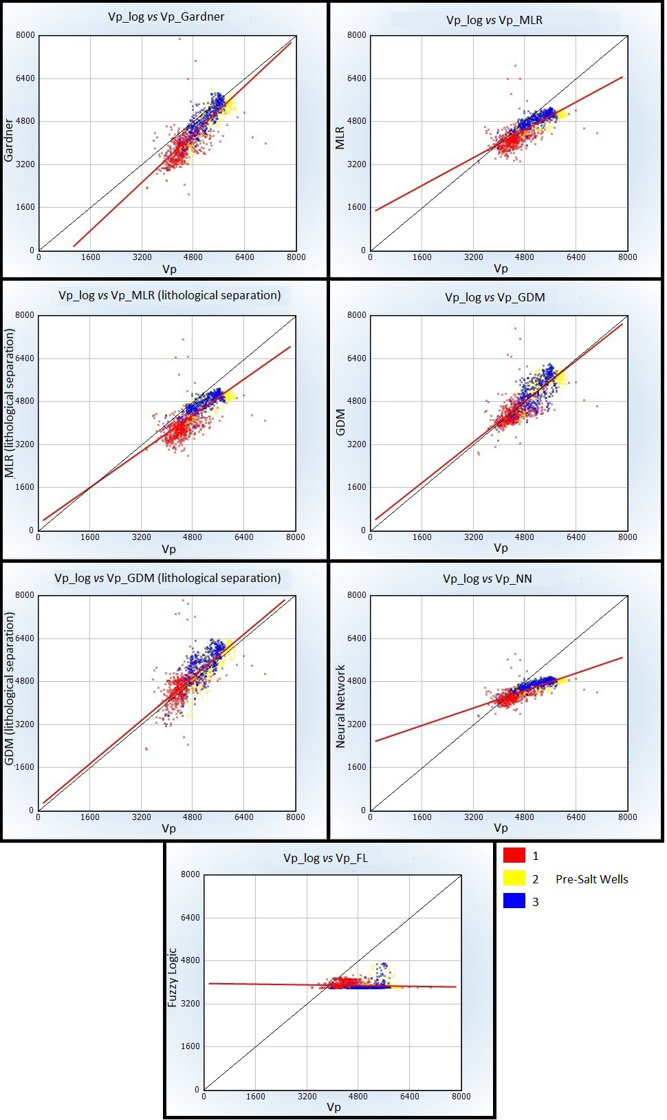
The results were plotted on real Vp vs. simulated Vp graphs for the different methods in all 57 wells used, and the results are shown in Figure 5. The crossplots contain the adjustment line (red) and their respective determination coefficients (R2), which are presented in Table 3. The equations of the adjustment lines are shown in Table 1, while Table 2 shows the Pearson Correlation coefficients (R) and Table 4 the Root Mean Square Error (RMSE).
In general, it can be observed that the models of Multiple Linear Regression and Geological Differential Method had the best results, both in terms of R2 values and in relation to slope of the adjustment line, which approach 45 degrees, and in the RMSE values. It is noted that the values of the Determination Coefficient (R2) and RMSE of the Fuzzy Logic method are better than the Gardner model, but their results were worse, as seen in the graphs of Figure 5, in which the slope of the adjustment lines shows that Gardner approaches more than 45 degrees, and observed in the logs plotted in Figures 2-4. This can be explained by the low variability of the simulation by Fuzzy Logic, whose values are always close to the real, but without expressing the lithological variations.
In relation to the application of the separation between siliciclastic and carbonate rocks in the MLR and GDM models, slightly better results were observed, with a small increase in R2 values, RMSE reduction and approximation of the adjustment line to the 45-degree slope. Considering that the methodology of separation of these lithologies is simple and that can be improved, the results can be even better.
| Gardner | Vp-Gardner = 656.684 + 0.78762 Vp |
| MLR | Vp-MLR = 1061.54 + 0.706433 Vp |
| MLR (Lithology) | Vp-MLR (Litho) = 858.997 + 0.761371 Vp |
| GDM | Vp-GDM = 581.868 + 0.849778 Vp |
| GDM (Lithology) | Vp-GDM (Litho) = 453.281 + 0.884034 Vp |
| Neural Network | Vp-Neural = 1887.43 + 0.506964 Vp |
| Fuzzy Logic | Vp-Fuzzy = 1506.96 + 0.580693 Vp |
Table 1: Equation of the adjustment lines of the real VP versus simulated VP graphs in all 57 wells used in Figure 5.
| Wells | Gardner | MLR | MLR (Lithology) | GDM | GDM (Lithology) | Neural Network | Fuzzy Logic |
|---|---|---|---|---|---|---|---|
| 57 (Total) | 0,74 | 0,85 | 0,88 | 0,84 | 0,89 | 0,71 | 0,83 |
| 3 Pre-salt wells | 0,77 | 0,79 | 0,80 | 0,80 | 0,77 | 0,80 | -0,06 |
| Pre-salt well 1 | 0,34 | 0,45 | 0,42 | 0,45 | 0,48 | 0,49 | -0,06 |
| Pre-salt wells 2 and 3 | 0,82 | 0,73 | 0,76 | 0,71 | 0,72 | 0,74 | 0,19 |
| Pre-salt well 2 | 0,81 | 0,67 | 0,69 | 0,72 | 0,75 | 0,70 | 0,11 |
| Pre-salt well 3 | 0,86 | 0,80 | 0,82 | 0,69 | 0,72 | 0,79 | 0,30 |
Table 2: Table with values of the Pearson Correlation Coefficients (R).
| Wells | Gardner | MLR | MLR (Lithology) | GDM | GDM (Lithology) | Neural Network | Fuzzy Logic |
|---|---|---|---|---|---|---|---|
| 57 (Total) | 0,55 | 0,72 | 0,77 | 0,71 | 0,73 | 0,51 | 0,69 |
| 3 Pre-salt wells | 0,59 | 0,63 | 0,64 | 0,64 | 0,60 | 0,64 | 0,004 |
| Pre-salt well 1 | 0,12 | 0,20 | 0,18 | 0,21 | 0,24 | 0,24 | 0,004 |
| Pre-salt wells 2 and 3 | 0,68 | 0,53 | 0,58 | 0,51 | 0,51 | 0,54 | 0,04 |
| Pre-salt well 2 | 0,65 | 0,45 | 0,47 | 0,52 | 0,57 | 0,49 | 0,01 |
| Pre-salt well 3 | 0,74 | 0,63 | 0,67 | 0,48 | 0,52 | 0,63 | 0,09 |
Table 3: Table with values of the Determination Coefficients (R2).
| Wells | Gardner | MLR | MLR (Lithology) | GDM | GDM (Lithology) | Neural Network | Fuzzy Logic |
|---|---|---|---|---|---|---|---|
| 57 (Total) | 594,6 | 416,0 | 376,2 | 448,9 | 429,4 | 578,1 | 453,1 |
| 3 Pre-salt wells | 678,8 | 494,3 | 653,7 | 390,6 | 479,4 | 573,5 | 1242,3 |
| Pre-salt well 1 | 946,9 | 522,6 | 801,5 | 449,5 | 530,4 | 421,1 | 724,1 |
| Pre-salt wells 2 and 3 | 442,5 | 476,2 | 544,7 | 349,9 | 445,6 | 648,9 | 1470,6 |
| Pre-salt well 2 | 480,7 | 545,3 | 603,3 | 302,6 | 400,1 | 727,8 | 1571,7 |
| Pre-salt well 3 | 398,6 | 391,2 | 475,6 | 393,4 | 488,7 | 554,3 | 1356,8 |
Table 4: Table with Root Mean Square Error (RMSE) values.
Pre-Salt Wells-Blind Test
The results of the simulations of the 3 pre-salt wells, which served as blind test, are shown in Figures 6-9 shows the graphs of real VP versus simulated VP for the 3 wells of the pre-salt and in its equations of the adjustment lines in Table 5. By analyzing the logs of the 3 wells, different characteristics of well 1 can be observed in relation to wells 2 and 3, which may be related to the location of these wells. Well 1 is in a different field from the others. It presents high gamma radioactivity to the carbonate rock patterns, which may have caused poor simulations performance in this well.
The curves simulated by Fuzzy Logic presented very
poor results, as well as in the post-salt wells, as can be seen in Figures 6-9 and in Tables 2-5. Meanwhile, the Neural Network simulation obtained good results in terms of values of R2 and RMSE, but it is observed that the adjustment line is very distant from the ideal slope of 45 degrees. Like what was observed in the general analysis (57 wells) for the simulation by Fuzzy Logic, which can be explained by the smaller variability of the simulated curve by Neural Network.
The Gardner models and Geological Differential Method (GDM) had a good correlation with the original curve, both in terms of R2 (Table 3) and RMSE (Table 4) values, as well as in a visual analysis of the plotted logs and the slope of the adjustment line in cross plots.
As mentioned previously, well 1 of the pre-salt has distinct characteristics and thus none of the models obtained satisfactory R2 values when the well was analyzed alone. However, when analyzing the plotted logs, there is a great similarity with the real log, especially the GDM and Neural Network.
Considering only the wells 2 and 3, the Gardner method obtains higher values of R2, in addition to approaching the real profile when plotted. However, the GDM method presents an inclination of the adjustment line very close to 45 degrees, besides showing a lower RMSE value, being considered the best prediction method in the 3 wells of the blind test.
Contrary to the general analysis, the application of siliciclastic and carbonate rock separation in the MLR and GDM models did not show a consistent improvement of the results.
| Gardner | Vp-Gardner = -1033.84 + 1.12025 Vp |
|---|---|
| MLR | Vp-MLR = 1376.77 + 0.650739 Vp |
| MLR (Lithology) | Vp-MLR (Litho) = 236.833 + 0.842593 Vp |
| GDM | Vp-GDM = 249.421 +0.948353 Vp |
| GDM (Lithology) | Vp-GDM (Litho) =124.128 + 1.00591 Vp |
| Neural Network | Vp-Neural = 2525.17 + 0.404884 Vp |
| Fuzzy Logic | Vp-Fuzzy = 3968.34 + 0.0172339 Vp |
Table 5: Equations of the adjustment lines of the real Vp versus simulated Vp graphs in the pre-salt wells shown in Figure 9.
Conclusions
The P wave velocity log simulations showed that the model of Gardner, et al. [5] produces good results for the Campos Basin and Santos Basin pre-salt wells but presents a lower correlation with the real log in regions of higher porosity, because that greater presence of fluid causes in the well logs, and also in some shale intervals. This effect was not observed in the other models, since they use, in addition to the density log, the resistivity and gamma ray logs to predict Vp, thus softening the alterations suffered by the logs in these regions.
The simulated models, Fuzzy Logic (FL) and Neural Network (NN), did not have good results, although in some analyzes of correlation with the real log, similar or better values of Coefficient of Determination (R2) and Root Mean Square Error (RMSE) than the other methods. This happened due to the low variability of these simulated curves, being little representative for the lithological changes.
In a general analysis, with all 57 wells used in the study (54 model wells and 3 blind wells), the Multiple Linear Regression (MLR) method proved to be the most efficient, followed by the Differential Geological Method (GDM). It was also observed a slight improvement in the correlations for these models when simulated using the separation between siliciclastic and carbonate rocks.
When analyzing only the 3 wells of the Santos Basin pre- salt (blind test), the GDM model obtained the best results, followed by the Gardner, et al. [5] and MLR. In the pre-salt well 1, none of the methods presented satisfactory R2 value, although the Neural Network and GDM methods presented low RMSE values and similarity with the original curve when plotted. This is believed to have occurred because of the peculiar feature of this well, which shows values of the gamma ray log above the carbonate pattern.
In general, the GDM method presented the best results, followed by the Gardner and MLR methods. The three methods demonstrated the capability to simulate the Vp log when it is not available. Gardner has the advantage of using only the density log, while the others require that the gamma rays and resistivity profiles are also available.
Acknowledgments
We thank UENF-LENEP for their physical and computational infrastructure, CNPq by the research grant, Petrobras, and Petrogal Brasil S.A. by the support to develop this study, LR Senergy for software academic license, Petrobras/ANP/UENF covenant for data set, grant and fees.
References
-
Augusto F, Martins J (2009) A well-log regression analysis for p-wave velocity prediction in the Namorado Oilfield, Campos Basin. Brazilian Journal of Geophysics 27(4): 595-608.
-
Islam N (2011) Sonic log prediction in carbonates. Master’s Thesis, _Michigan Technological University,_ Houghton, MI, USA, pp: _91._
-
Leite M, Carrasquilla A, Da Silva J (2008) Simulation of the sonic log from the gamma rays and resistivity logs in wells in the Campos Basin. Brazilian Geophysical Journal 26(2): 141-151.
-
Cao J, Shi Y, Wang D, Zhang X (2017) Acoustic log prediction based of kernel extreme learning machine for wells in gjh survey, erdos basin. Journal of Electrical and Computer Engineering 3824086.
-
Gardner G, Gardner L, Gregory A (1974) Formation velocity and density - the diagnostic basics for stratigraphic traps. Geophysics 39(6): 770-780.
-
Faust L (1953) A velocity function including lithologic variation. Geophysics 18(2): 271-288.
-
Lorenzen R (2018) Multivariate linear regression of sonic logs on petrophysical logs for detailed reservoir characterization in producing Fields. Interpretation 6(3): T531-T541.
-
Bukar I, Adamu M, Hassan U (2019) A machine learning approach to shear sonic log prediction. SPE Nigeria Annual International Conference and Exhibition, Lagos, Nigeria.
-
Hatampour A, Ghiasi-Freez J (2013) A fuzzy logic model for predicting dipole shear sonic imager parameters from conventional well logs. Petroleum Science and Technology 31(24): 2557-2568.
-
Ramos M, Martins J, Bijani R (2017) Analysis and validation of two mathematical models of acoustic impedance in well logs: an example in Namorado oilfield, Campos basin, Brazil. Journal of Petroleum Science and Engineering 158: 739-750.
-
Silva M, Santos R, Martins J, Fontoura S (2002) Prediction of P-wave sonic logs via neural network and seismic trace inversion: a comparison. Offshore Technology Conference, Houston, Texas, USA, pp: 1-7.
-
Senergy LR (2021) Interactive Petrophysics Software Ltd.
-
Chatterjee S, Simonoff J (2013) Handbook of regression analysis. International Statistical Review 81(2): 330- 331.
-
Zakaria M, Mabrouka AS, Sarhan S (2014) Artificial neural network: a brief overview. Journal of Engineering Research and Applications 4(2): 7-12.
-
Hurst A, Tischler GE, Arkalgud R (2009) Predicting reservoir characteristics from drilling and hydrocarbon- gas data using advanced computational mathematics. SPE, Offshore Europe Oil and Gas Conference and Exhibition, Aberdeen, UK, pp: 248-257.
-
Tischler G, Arkalgud R, Hurst A (2006) Prediction of petrophysical characteristics from borehole gas and drilling data. 68th EAGE Engineers Conference and Exhibition, incorporating SPE EUROPEC 2006: Opportunities in mature areas, Vienna, Austria, pp: 3091-3095.
-
Hayton S, Tischler G (2014) Getting back to basics: Using routine drilling mud logging data for reservoir characterization. SPE/EAGE European Unconventional Resources Conference and Exhibition, Austria.
-
Huber-Carol C, Balakrishnan N, Nikulin N, Mesbah M (2002) Goodness-of-Fit Tests and Model Validity. 1st(Edn.), Statistics for Industry and Technology, Birkhäuser, Basel, pp: 507.
- Nigeria’s Vulnerability in the Face of Global Energy Policy
- A Simulation Study of Investigation of Optimum Oil Production Performance by Applying Various Gas Injection Methods in Oil Reservoir
- Characterization of Permo-Triassic Reservoirs through Thermal Maturity Assessment of Westphalian Source Rocks in the Cheshire Basin
- Influence of Microwax on the Rheological and Thermal Behaviour of a Wax Crude Oil
- Real-Time Monitoring and Performance Optimization of Steam Injection in Heavy Oil Reservoirs Using Fiber Optic Sensing and Integrated Predictive Simulation Models
- Rapid On-Site Determination of the Total Petroleum Hydrocarbon Content of Soils by Handheld Fourier Transform Near-Infrared Spectroscopy: Development of a Global, Site- and Scanner- Independent Calibration Model