Optimization of Drilling Cost Using Artificial Intelligence
Drilling operations in the oil and gas industry takes most of the well cost and how fast the drilling bit penetrate and bore the formation is termed the Rate of penetration (ROP). Since most of the cost incurred during drilling is related to the drilling operations, there is need not only to drill carefully, but also to optimize the drilling process. A lot of parameters are related to the rate of penetration which are actually interdependent on each other. This makes it difficult to predict the influence of every single parameter Drilling optimization techniques have been used recently to reduce drilling operation costs. There are different approaches to optimizing the cost of drilling oil and gas wells, some of which include static and /or real time optimization of drilling parameters. A potential area for optimization of drilling cost is through bit run in the well but this is particularly difficult due to its significance in both drilling time and bit cost. In this sense, as a particular bit gets used, it gets dull as its footage increases, resulting from the reduction in the bit penetration rate. The reduction in penetration rate increases total drill time. In order to optimize bit cost, it is desirable to find a trade-off between the two by a bit change policy This study is aimed at minimizing drilling time by use of artificial intelligent for the bit program. Data obtained from a well in the Niger delta region of Nigeria was used in this study and the cost optimization modelled as a Markov decision process where the intelligent agent was to learn the optimal timings for bit change by reinforcement policy Iteration learning. This study was able to achieve its objectives as the reinforcement learning optimization process performed very well with time as the computer agent was able to figure out how to improve drilling cost over time. Better results could be obtained with a better hardware and increased training time.
Introduction
Since drilling costs represent a major fraction of total exploration and production costs. Reduction in operations cost will impact the total time spent will drilling a well. As a result the ability to optimize drilling costs would not only encourage exploration for more reserves but also increase profitability even with the present low oil price making Oil and gas more competitive as an energy source. Although there are many methods of optimizing drilling cost most if not all of which depend on the ability to accurately predict penetration rate. Thus it is very important to be able to accurately predict ROP especially for directional wells.
Penetration rate is difficult to predict accurately especially for directional wells. This in turn makes cost optimization difficult. A potential area for optimization of drilling cost is bit use. This is particularly difficult due to its significance in both drilling time and bit cost. In this sense, as a particular bit gets used, it gets dull as its footage increases. The dullness of the bits affects its penetration rate. The reduction in penetration rate increases total drill time. Hence early changing of bits reduces drill time at the expense of bit cost. While late bit changes increase drill time while minimizing bit use. In order to optimize bit cost, it is desirable to find a trade-off between the two by a bit change policy to reduce cost.
Cost Optimization is a procedure which involves finding the most cost effective alternatives under a given set of constraints by maximizing desired factors and minimizing undesired ones. By extension, drilling cost optimization involves finding the most cost effective combination of drilling parameters in other to minimize drilling time and consequently drilling cost. Most drilling cost optimization techniques rely on the ability the accurately predict Rate of penetration or penetration rate. Hence a lot of work has been done to develop accurate rate of penetration models. The cost per footage drilled is given by the general equation 1.
( ) 1 / d b C R t C F = + + (1)
Where C = Total cost per footage drilled($/ft), R = Rig Operating Cost($/hr), t = total trip time(hrs), td = total drilling time(hrs), Cb= Total bit cost (hrs), F = Footage drilled(ft) The Rig operating cost is known as well as the footage drilled, the total drill time depends on the Penetration rate. For a given footage drilled, the total time can be expressed as shown in the equation 2.
0 1/ f t ROP =∫ (2)
Where t is the total drill time (hrs), ROP = Penetration rate (ft/hr) and f= footage drilled.
In recent times, drilling rate optimization techniques have been used to reduce drilling time which invariably translate to reduced cost of drilling. However Rate or penetration (ROP) which is the rate at which the drill bit deepens the well beneath usually reported in units of feet/hour is a complex non-linear function of various drilling parameters such as: Weight on Bit(WOB), Rotational speed (Revolutions per minute or N) flowrate(Q), bit diameter, bit tooth wear, bit hydraulics, formation strength, and formation abrasiveness. Given this complex non-linear relationship between Rate of Penetration and these variables, it is extremely difficult to develop a complete mathematical model to accurately predict ROP from these parameters.
Several ROP models have been proposed. Among these models, the most well-known ones are Burgoyne and Young, and Warren’s models. However, they did not provide satisfactory accuracy. In each of these models different parameters have been used to estimate the ROP. With advances in computer technology, Artificial neural networks are capable of learning the relationship between these parameters and Rate of penetration given a large enough data set, trained network can hence be used to predict ROP from the above parameters. An ‘artificial’ neural network (ANN), is a processing devices (algorithms or actual hardware) that are loosely modeled after the neuronal structure of the mammalian cerebral cortex but on much smaller scales. Once a neural network is ‘trained’ to a satisfactory level it may be used as an analytical tool on other data. Reinforcement Learning is a type of Machine learning and consequently artificial intelligence that allows a computer agent without being explicitly programmed to learn in a specific context, the ideal behavior or strategy to maximize its performance by making use of a simple reward feedback thereby maximizing rewards.
Reinforcement learning has been used in recent times to achieve state of the art technological breakthroughs including computer programs learning how to play certain games at a superhuman levels and in self driving cars. The first step in reinforcement learning is to design/develop the decision making environment for the environment to learn. The environment is modelled as a Fully Observable Markov Decision Process (MDP).
Value of A Policy
The expected value of a policy π for the discounted reward, with discount γ, is defined in terms of two interrelated functions, Vπ and Qπ. defined recursively in terms of each other.
Let Qπ(s,a), where s is a state and a is an action, be the expected value of doing a in state s and then following policy π, and Vπ(s), where s is a state, expected value of following policy π in states.
If the agent is in state s, performs action a, and arrives in state s’, it gets the immediate reward of R(s,a,s’) plus the discounted future reward, γVπ(s’). When the agent is planning it does not know the actual resulting state, so it uses the expected value, averaged over the possible shown in the equation 3 , Q (s,a)= P(s'|s,a) [R(s,a,s')+ V (s' )] s π π γ ∑ (3) Vπ(s) is obtained by doing the action specified by π and then acting following π:
V (s)= Q (s, (s)) π π π (4)
Value of an Optimal Policy
Let Q*(s,a), where s is a state and a is an action, be the expected value of doing a in state s and then following the optimal policy. Let V*(s), where s is a state, be the expected value of following an optimal policy from state s. Q* can be defined analogously to Qπ as presented in the equation 5.
[equation]
(5) V*(s) is obtained by performing the action that gives the best value in each state as can be seen in the equation 6.
a V*(s) = max Q*(s,a) (6)
An optimal policy π* equation 7, is one of the policies that gives the best value for each state:
a ð*(s) = argmax Q*(s,a) (7)
MDP Solution Methods
Value Iteration
The Value iteration starts with an arbitrary function V0 and using the following equations 8 and 9 to get the functions for k+1 stages to go from the functions for k stages.
[equation]
(8) k a k V (s)= max Q (s,a) for k>0 (9)
Policy Iteration
The Policy iteration starts with an arbitrary policy π0 (an approximation to the optimal policy works best) and iteratively improves it. A lot of works have been done in the area of predicting penetration rate from drilling and optimizing parameters with the objective of maximizing footage drilled and minimizing drilling cost simultaneously. This optimization is usually achieved by varying any of the drilling parameters particularly weight on bit and rotation speed. One of the first attempts for the drilling optimization purpose was presented in the study of Graham and Muench [1]. They analytically evaluated the weight on bit and rotary speed combinations to derive empirical mathematical expressions for but life expectancy and for drilling rate as a function of depth, rotary speed and bit weight. Maurer [2] derived rate of Penetration equation for roller-cone type of bits considering the rock cratering characteristics. The equation was based on perfect hole cleaning condition where all the debris is considered to have been removed between the tooth impacts. A working relation between drilling rate, weight on bit, and string speed was achieved assuming that the hole was subject to perfect hole cleaning circumstances. It was also mentioned that the obtained relationships were a function of drilled depth. Bingham [3] proposed a rate of penetration equation based on laboratory data, In the equation the threshold bit weight was assumed to be negligible and rate of penetration a function of applied weight on the bit and rotary speed of the string. The bit weight exponent, a, was set to be determined experimentally through the prevailing conditions.
Some early studies performed in regards to optimal drilling detection was by Bourgoyne and Young [4], They constructed a linear penetration rate model and performed a multiple regression analysis of drilling data in order to select the optimum bit weight rotary speed, and bit hydraulics.. They found that regression analysis procedure can be used to systematically evaluate many of the constants in the penetration rate equation. Warren [5] presented an ROP model that includes the effect of both the initial chip generation and cuttings removal process. The rate of penetration equation they derived is formed of two terms, working only with perfect hole cleaning assumption. The first term defined the maximum rate supporting the WOB effect without tooth penetration rate, the second term on the other hand considering bit penetration into the formation. In recent years drilling parameters are easily acquired, stored and also transferred in real time basis. A range of drilling optimization and control services started to take place with the introduction of sophisticated and automated rig data. Maidla and Ohara [6] tested a drilling model on offshore drilling data and compared their findings with the Bourgoyne and Young’s model. Their result was that ROP for successive wellbores in the same area could be predicted based on the coefficients calculated from the past drilling data, resulting in cost savings. They concluded that the drilling model performances depended on the quality of the data used to conduct the syntheses and presented isocost, iso-ROP graphs for cost effective drilling activities. Ursem, et al. [7] demonstrated how an operator and a service company illustrated the use of latest technology within the scope of Real Time Operations centre. They performed some pilot tests on exploration wells which revealed communications improved interventions and made the advices much more clear, limiting downtime. Eren, et al. [8] conducted a multiple regression analysis to find the regression coefficients of the pre-defined general ROP model in order to predict ROP. This gives the flexibility of ROP follow-up as a function of drilling parameters specifically for subject formation. The modelled ROP prediction showed realistic match with the actual observations. The predicted ROP trend could be compared in real-time with what actually is occurring.
Monazami, et al. [9] presented an application of Artificial Neural Network (ANN) methods for estimation of ROP among drilling parameters obtained from one of Iranian southern oil fields, according to the fact that this method is useful when relationships of parameters are too complicated. The method is proposed as a more effective prognostic tool than are currently available procedures. The methodology enables. The network was trained from 336 cases collected from the daily drilling reports in one of the southern Iranian oil fields. Wanyi Jiang [10] used a combination of Artificial Neural Networks (ANN) and Ant Colony Optimization(ACO) to determine optimal Rate of Penetration. The Bayesian regularization neural network was trained using the modified Warren model for ROP for rolling cutter bits. The ACO algorithm was then used to optimize the drilling parameters by brute force. Akintola and Ojuolapel [11] investigate drilling cost optimization for Extended Reach Deep Wells Using Artificial Neural Networks, the result from their study showed the Normalized Rate of Penetration (NROP) more accurately identifies the formation characteristics thereby reducing drilling. This study is aimed at optimizing drilling cost by developing an algorithm that intelligently plans and schedules bit replacement to minimize drilling time with as few bits as possible. Data from a directional well in the Niger Delta region of Nigeria is used in this study. The daily drilling reports from the field were collected, cleaned and used.
Materials and Methodology
The first step in optimizing rate of penetration is developing a reasonably accurate model relating drilling parameters to rate of penetration. This model can then be optimized by a number of numerical or computer algorithms. Being that rate of Penetration is a complex non-linear function of several variables, and also these independent variables are not particularly defined. Different variables have made use of slightly different independent variables. These make it difficult to build a particularly accurate mathematical model. Statistical methods have hence been looked into to build the best possible approximations of Rate of Penetration models. A deep regression neural network using JAVA’s open source machine learning program DL4J. was used to develop this model, drilling reports were obtained from a directionally drilled well in the Niger Delta. The drilling reports spanning a period of two months containing all activities performed by the drilling contractors was obtained and the necessary data for the development of the model was extracted The following independent parameters: Inclination angle (Directional well) Mud pump( gpm), Minimum Weight on bit(KIPS), Maximum weight on bit(KIPS), Drill string (rpm), Mud weight (ppg), % Sand in mud, Depth (in), Depth out (ft),Bit Diameter(in), Depth previously drilled by bit, Torque, Slack off weight and Rotating weight were chosen for the 58 case studies:
Pre-Processing of Data: The pre-processing was carried out with the normal MinMAx scaler in the dl4j library and all the input Data Were First Normalized to Values Between 0 And 1 With The Targets Also Scaled (Normalized). Model Architecture: Some of the important architectural decisions made include: Number of hidden layers, Number of units in each layer, learning rate, loss function for each layer, activation function for each layer, Weight initialization system, Weight updater, Number of epochs, The model was than trained several times with a lot of tweaks and the differences in results were observed using different hyper- parameters. The eventual choices of hyper parameters were: Number of input neurons-12; Number of hidden layers-3, Number of neurons per hidden layer -10; Learning rate -0.01, Updater – NESTEROVS, Momentum- 0.9, Layer 1,2,3 activation – RELU, Layer 4 activation – Identity, and Output layer loss function – Mean Square error The model was trained with 50 data points and tested with 8.
Training the Network
In order not to overtrain’ the model, the data set was split into the training set and the test set. A batch size of 64 was set so that the full data passes in a single batch, With the number of epochs set to 20,000 at one iteration per epoch, the number of iterations was equal to 20,000. In order to observe the performance of the network during training. The evaluation statistics were: Iteration score- Mean Square Error of the train set, Mean Absolute Error of the test set, Mean Square Error of the test set, Root mean square error of the test, the coefficient of regression (R2)
Tuning the Model to Improve Accuracy
The model was adjusted severally, based on the model performance observed during the training with some important hyper parameters tweaked
Developing an Optimization Model
A directional well drilled in the Niger Delta region of Nigeria was used as case study, the aim was to develop a bit replacement schedule to reduce significantly the cost of drilling the well. In order to carry this out, the approach required must be intelligent enough to consider the long term effects of its actions.
Modelling the Drilling Optimization MDP
From the daily drilling reports, the different trip depths were recorded as the decision points where the agent choses to either continue or change the bit. The states are defined by the following parameters: Entry Depth, y1, Current depth, y2, Footage previously drilled by bit, y; Bit number, n and Time spent. The decision process started at a depth of 6315 feet when the 12 ¼ bit was inserted up to the total depth of 11812 feet. There was a total of 42 trips and consequently 42 decisions to be made. In mathematical terms, there are two decisions to pick from 42 times leading to a total of 242 (4.4 X 10¹²) possible permutations which makes this problem very computationally difficult. The MDP was developed with BURLAP, a Java Artificial Intelligence framework as a deterministic Decision making problem (Deterministic in the sense that the probability for each transition is set to 1) (Figure 1).
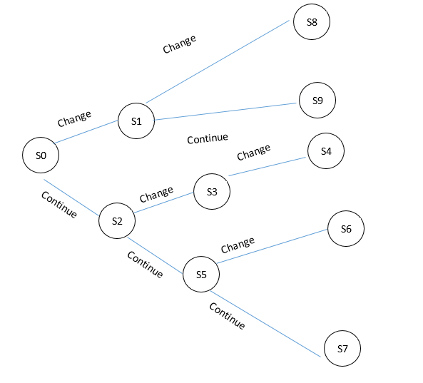
At every decision point, the ‘changebit’ action causes the next state to have a y value of zero while y1 becomes y2 of the previous state, y2 becomes the next trip depth. The ‘Continue’ action computes i.e accumulates the drilled footage for the next state while updating y1 and y2 as in the ‘change bit’ action. In either case, to determine and update the time parameter, the ROP two layered neural network previously developed to fit the well is used to compute the average penetration rate for the state. The time expended is then computed as (y2-y1)/ROP. Then the time is added to the previous cumulative time expended.
Reward Function
The reward was set to zero for all states apart from the final depth. At the final depth, The total cost to drilling depth ignoring trip time is computed using the equation 10.
( ) ( ) bit rig C n C Cost time = × + × (10)
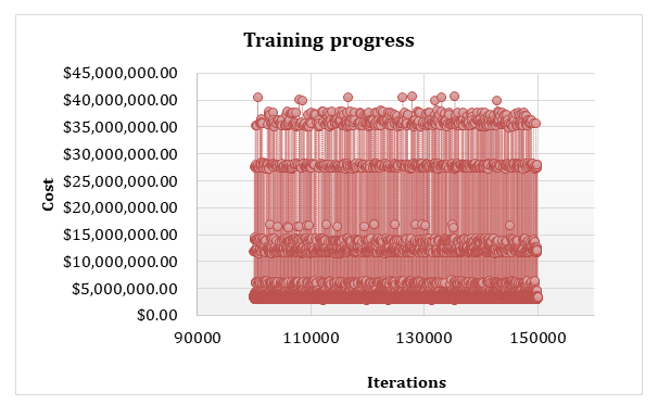
From the equation 10, it is observed that optimizing C involves a tradeoff between time and number of bits, using more bits causes the well to be drilled faster at the expense of bit cost. The MDP was set up as shown in Figure 1 and then solved by policy iteration over 160000 iterations to determine the optimal bit number, bit change depths and cost.
Assumptions and Simplifications
- Trip time was modelled as a linear function of depth
- A bit cost of $50,000 and a rig cost of $7000/hour were used
- The trip depths were maintained as in the original drilling operation
MDP Solution with Q-Learning Algorithm
The Q values were initialized for all state action pairs arbitrarily, the learning rate and a number of iterations were selected for each iteration; starting from the initial state, the agent selects an action following an epsilon greedy policy using Q values for state action pairs. The reward r and next state, s’ observed from taking action a from state s are noted and the Update Q value is presented in the equation 11.
( ) ( ) ( ) ( ) , , , ', ' , a Q s a Q s a R max Q s a Q s a α γ ⇐ + + − (11) This was repeated until the terminal state and different combinations of learning rate, number of iterations and initial Q values were experimented with.
Results and Discussion
It was observed from the results for the Penetration rate prediction using the neural network architectures that there were trained with a single layer, two hidden layers, and three hidden layers. All layers had 10 hidden units per layer with an Optimization Algorithm- Stochastic Gradient Descent. The single layers had 20,000 iterations and 50,000 iterations for both two and three hidden layers. Their learning rate was 0.01 for single layer and 0.0065 for both two and three hidden layers. The momentum was 0.9 for single layer and 0.8 for both two and three hidden layers. Both the two and three hidden layers had RELU Activation function except for output layer, with Identity Activation function.
The result for the single hidden layer network is shown in the Figure 2. That for two hidden layers network training and test are presented in the Figures 3 & 4, respectively, while the same result for the three hidden layers presented in the Figures 5 & 6 respectively.
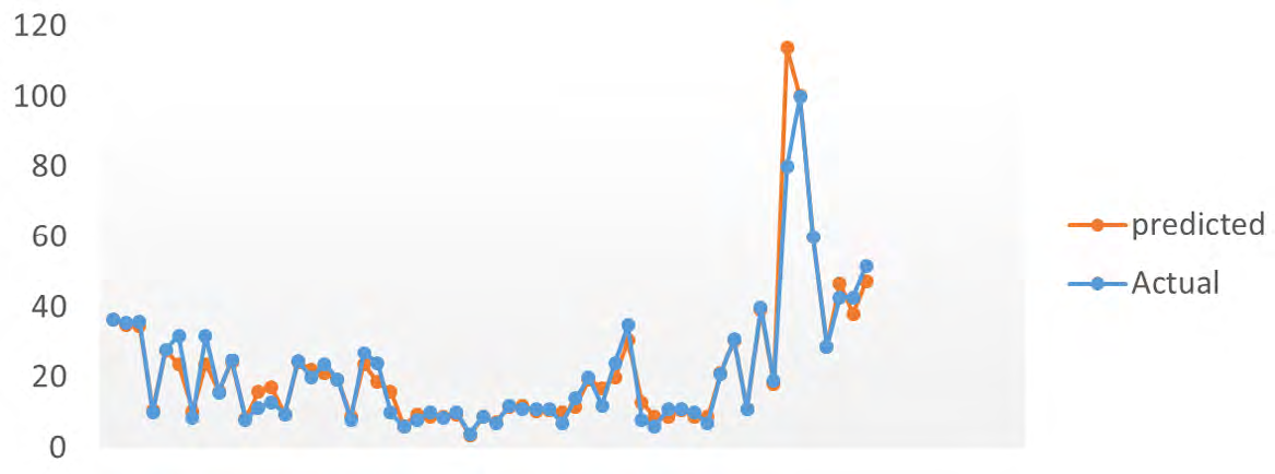
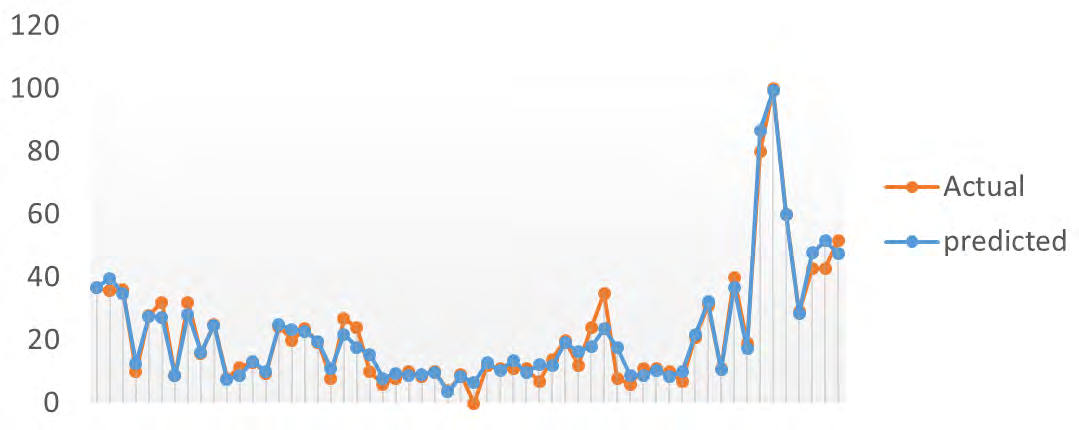
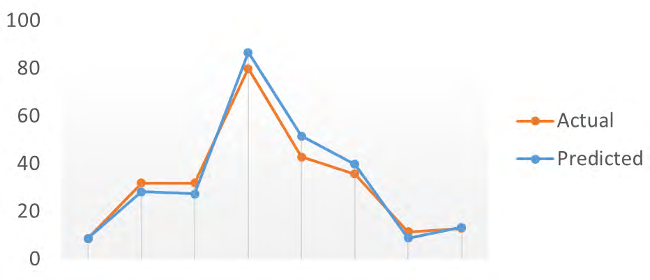
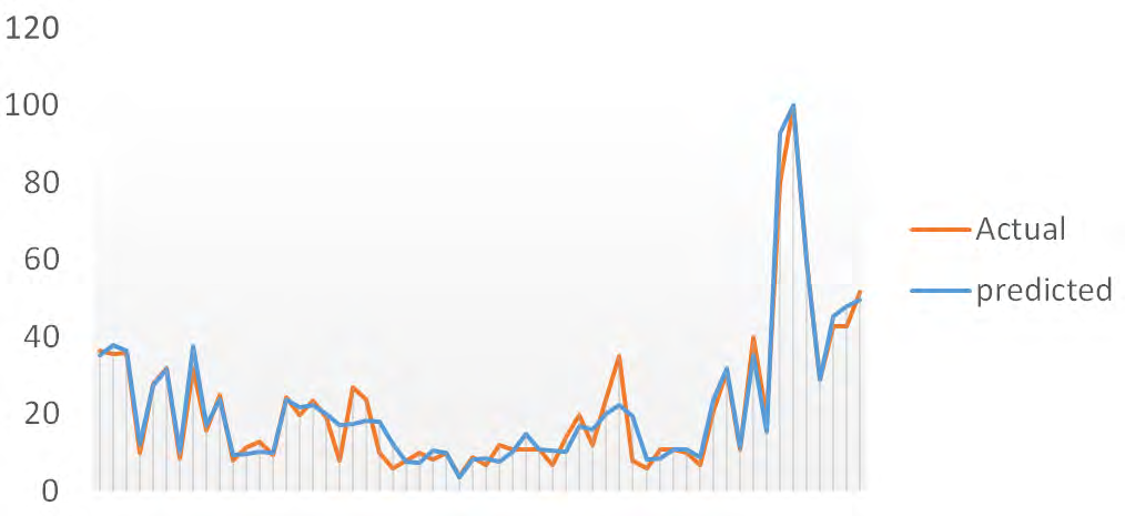
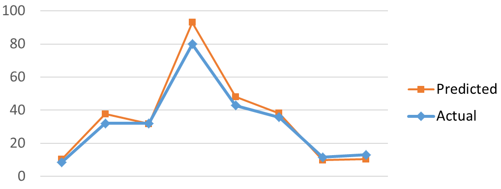
The Table 2 presents the summary of the statistical result of the training network for all the hidden layers from the result it can be seen that the two hidden layered neural network produced the best results, thus it would be used for further optimization work.
| Hidden Layers | MSE | MAE | R | MSE(test) | MAE(test) |
|---|---|---|---|---|---|
| One | 27.56 | 2.4 | 0.975 | 168.5 | 8.28 |
| Two | 12.485 | 2.44 | 0.992 | 22.865 | 3.88 |
| Three | 18.29 | 2.92 | 0.992 | 30.6 | 4.06 |
Table 1: Results Summary.
Reinforcement Learning
The following parameters were used for the reinforcement learning: minimum cost recorded - $2,876,895, number of bits used – 10,,Total Drill time – 340 hours, Bit change depths: 6670 ft., 6703ft., 7570 ft., 8396 ft., 8409 ft., 8883 ft.,
9897ft., 10372ft., 10793ft (Figure 7).
Using the actual drilling data: cost = $3,010,700, number of bits used – 9; Drill time – 365 hours and cost saved = $133,805.
The results of this study indicate the following: 1. The Neural network models are able to predict Penetration rate with very high accuracy 2. The system was able to learn over time by reinforcement learning how to reduce cost by optimizing bit use.
3. The results of the model were determined by the choice of bit cost and drilling cost rate 4. This model was simplified by making it deterministic. Further precision can be obtained by introducing the stochastic nature of trip time and other factors
5. By repeating this experiment, with bigger data and larger computational power, and some of the simplifications taken off, we would be able to develop a drilling system with an automated decision maker better than humans
Conclusions
As oil and gas companies continue to explore and drill deep and ultra-deep water zones for hydrocarbons, there is an increasing need to have reduce personnel on board by automating as much as possible. This approach of training an intelligent agent to make decisions regarding bit change can replace and has been shown to be slightly more cost effective. In this study, the agent was shown to get better and more efficient with increasing iterations. With improved hardware and a more robust model involving much more samples and better bit wear models, much better agents can be developed and deployed for different drilling implications. This study also shows how reinforcement learning can be used to replace human intuition in decision making and can be extended to other oil and gas applications.
Lastly, it was shown that with good architecture and feature engineering, neural networks can be used to predict with groundbreaking accuracies Penetration rates in deviated wells and this can be applied to subsequently most other functional relationships in oil and gas.
References
-
Graham JW, Muench NL (1959) Analytical determination of optimum bit weight and rotary speed combinations. The fall meeting of the society of petroleum engineers, Dallas, TX, USA.
-
Maurer WC (1962) The perfect-cleaning theory of rotating drilling. J Pet Technol 14(11): 1270-1274.
-
Bingham MG (1965) A New Approach to Interpretting Rock Drillability. Oil and Gas Journal.
-
Bourgoyne A, Millheim K, Cenevert M, Young F (1986) Applied Drilling Engineering. Vol. 2, SPE Textbook series.
-
Warren TM (1987) Penetration Rate Performance of Roller Cone Bits. SPE Drill Eng 2(1): 9-18.
-
Maidla EE, Ohara S (1991) Field Verification of Drilling Models and Computerized Selection of Drill Bit, WOB, and Drillstring Rotation. SPE Drill Eng 6(3): 189-195.
-
Ursem LJ, Williams JH, Pellerin NM, Kaminski DH (2003) Real Time Operations Centers; The people aspects of Drilling Decision Making. SPE/IADC Drilling Conference, Amsterdam, Netherlands.
-
Eren T, Ozbayoglu ME (2010) Real Time Optimization of Drilling Parameters During Drilling Operations. The SPE Oil and Gas India Conference and Exhibition, Mumbai, India.
-
Monazami M, Hashemi A, Shahbazian M (2012) Drilling Rate Of Penetration Prediction Using Artificial Neural Network: A Case Study Of One Of Iranian Southern Oil Fields. Oil and Gas Business 6: 21-32.
-
Wanyi Jiang (2016) Optimization of Rate of Penetration in a Convoluted Drilling Framework using Ant Colony Optimization. IADC/SPE Drilling Conference and Exhibition, Fort Worth, Texas, USA.
-
Sarah A, Ojuolapel TT (2021) Drilling Cost Optimization for Extended Reach Deep Wells Using Artificial Neural Networks. Saudi Journal Engineering Technology 6(6): 118-129.
- Nigeria’s Vulnerability in the Face of Global Energy Policy
- A Simulation Study of Investigation of Optimum Oil Production Performance by Applying Various Gas Injection Methods in Oil Reservoir
- Characterization of Permo-Triassic Reservoirs through Thermal Maturity Assessment of Westphalian Source Rocks in the Cheshire Basin
- Influence of Microwax on the Rheological and Thermal Behaviour of a Wax Crude Oil
- Real-Time Monitoring and Performance Optimization of Steam Injection in Heavy Oil Reservoirs Using Fiber Optic Sensing and Integrated Predictive Simulation Models
- Rapid On-Site Determination of the Total Petroleum Hydrocarbon Content of Soils by Handheld Fourier Transform Near-Infrared Spectroscopy: Development of a Global, Site- and Scanner- Independent Calibration Model