Logarithm Model for Decline Curve Analysis
A decline curve analysis model has been developed for flow rate proportional to the logarithm of time. The logarithm of time model requires careful interpretation of initial time dependence of volumetric flow rate. Applications of the model to shale gas production and shale oil production are presented.
Introduction
A typical decline curve analysis (DCA) model expresses flow rate q as a function of time f(t) so that q = f(t) with a first order time derivative ( ) df t dq dt dt = . Arps JJ [1] decline curves are solutions of the equation
1 n dq aq dt + = − (1)
The factors a and n are empirically determined and are constant with respect to time t. The empirical constant n ranges from 0 to 1. The shape of the decline curve depends on the value of n as shown in Table 1. The term qi is initial flow rate.
| Decline Curve | n | q = f ( t) |
|---|---|---|
| Exponential | 0 | q=q e−at i |
| Hyperbolic | 0 < n < 1 | q=n1/(nat+q −n) i |
| Parabolic | 1 | q=1/(nat+q−1) i |
| q = f(t) | Constants | Flow Regime Examples |
| q=atn+b | a, b, n | Rate q proportional to tn Volumetric flow (n = 1) Linear flow (n = ½) Bilinear flow (n = ¼) |
| q=alntn+b | a, b, n | Rate q as function of ln tn Radial flow (n = 1) |
Table 1: Arps JJ [1] Decline Curves.
Decline curve analysis provides information which can be used to estimate cumulative production N. If we assume a functional relationship ( ) q f t = is known, cumulative production is the integral over flow rate q for a period of time that ranges from initial time t0 to final time t, thus ( ) 0 0 t t t t N qdt f t dt = = ∫ ∫ (2) As an example, cumulative production N for Arps exponential decline equation is − = = ∫ (3) t iq q N qdt a
0 where flow rate is integrated over time from initial rate qi at initial time t0 = 0 to rate q at time t. Time periods such as day, month and year need to be consistently applied. For more discussion of Arps equation and decline curve analysis, see Lee [2], Sun [3], Fanchi and Christiansen [4], Ezekwe [5], Panja and Wood [6].
Another way to infer the time dependence of flow rate is to consider different types of flow. Flow regime models provide different relationships between pressure drop and time. As a first approximation, well flow rate during primary depletion is proportional to pressure drop p ∆ where pressure drop is the difference in pressure i wf p p p ∆ = − between initial reservoir pressure ip and wellbore flowing pressure wf p . The relationship between flow rate and time can be obtained by writing productivity index / J q p = ∆
as q J p = ×∆ and replacing pressure drop with its time- dependent form for different flow models. Table 2 shows relationships between flow rate q and time t for some flow regime examples.
or The purpose of this paper is to develop a decline curve analysis model for flow rate proportional to logarithm of time ln t. This model is referred to here as the logarithm model (LNDM).
Logarithm Model (LNDM)
The radial flow relationship between flow rate and time in Table 2 suggests that flow rate q is proportional to the logarithm of time ln t in the form ln q a t b = + (4) where a, b are constant with respect to time and n = 1. The differential equation for the rate-time dependence in Equation (4) is obtained by calculating the time derivative ( ) ln d a t b dq a dt dt t + = = (5) Equation (5) is the differential equation for the logarithm model LNDM and is the analog of Equation (1). The general solution of Equation (5) is ln + where = -a ln q a t b b λ = (6) We have introduced the parameter λ to show how to make physical units consistent. To demonstrate this, substitute -a ln b λ = into Equation (6) to obtain ( ) a ln t a ln ln / q a t λ λ = − = (7) The units are consistent when λ has the unit of time so that / t λ is dimensionless. The slope a has the same unit as flow rate q and 0 a < for a flow rate that declines as time increases. The parameter λ is expressed in terms of a, b by ( ) exp / b a λ = − .
Cumulative Production and Economic Limit
Cumulative production for the logarithm model is given by the integral ( ) 0 ln N a t b dt τ τ = + ∫ (8) for the time interval 0 t τ τ ≤ ≤ . We solve the integral in Equation (8) using ln ln axdx x ax x = − ∫ to find
0 0 ln N a t t t bt τ τ τ τ = − + (9)
( ) ( ) ( ) 0 0 0 0 ln ln N a a b τ τ τ τ τ τ τ τ = − − − + − (10)
The maximum production time occurs when flow rate 0 q → since flow rate 0 q < when t τ > . We have the condition ( ) 0 ln q t a b τ τ = = = + (11) Solving for τ gives exp b a τ = − (12) The economic limit occurs at time econ τ τ ≤ .
An alternative economic limit can be set for a non-zero economic rate econ q using the following procedure. The time corresponding to the non-zero economic rate econ q is found using the equation ( ) ln econ econ econ q t t q a t b = = = + (13) The time corresponding to the economic limit econ t is then ( ) exp / econ econ t q b a = − (14)
Initial Condition of LNDM Model
The logarithm model LNDM requires a careful interpretation of volumetric flow rate as a function of time when t goes to 0. The usual initial condition for models such as the familiar Arps models in Table 1 uses flow rate q(t) at the beginning of the time period, that is flow rate at q(t = 0). In the case of the LNDM model, we cannot use ln(q(t)) at time t = 0.
An alternative approach that is suitable for the LNDM model is to recognize that volumetric flow rate data are typically reported as the average volume of fluid produced in a period of time. For example, the first volumetric flow rate may be the volume produced in a day, a month, or a year. If we choose to view the flow rate as the volume produced throughout the time period rather than an instantaneous rate at the beginning of the time period, then we can define an integral that begins at the completion of time period 1. In practice, we can use daily, monthly, or annual rates of production versus time and integrate over time beginning at the completion of the first time period rather than at the start of the first time period. Initial production rate, or IP, is the volume produced during the first time period divided by the duration of the time period.
Application of the LNDM Model using Linear Regression Analysis
The logarithm model LNDM is applied by first rewriting the model ln + q a t b = as a straight line y x = + α β where α is the slope and β is the intercept of the straight line. The relationships between models are , ln , , and = b y q x t a α β = = = (15) Linear regression analysis is used to fit rate versus time data to the straight-line model y x α β = + . Logarithm model LNDM parameters , , b α λ are then obtained from linear regression parameters , α β using Equation(15), namely ( ) , = , and = exp / a b b a α β λ = .
Example: LNDM Model of Shale Gas Decline
The LNDM model was used to forecast shale gas recovery for four major North American shale gas fields [7]: Barnett, Fayetteville, Haynesville, and Woodford. As an example, the LNDM parameters for a high flow rate gas well are a = -1.0 x 10⁴ and b = 1.5 x 10⁵. The LNDM model parameters were calculated using monthly gas production so time is expressed in months. The gas rate after 3 years of production is calculated at t = 36 months so that ( ) ( ) 4 = + × ×
5 5 ln b=-1.0 10 ln 36
q a t (16) + × = ×
1.5 10 1.14 10 / MSCF mo
Application of the Logarithm Model to Shale Gas Production
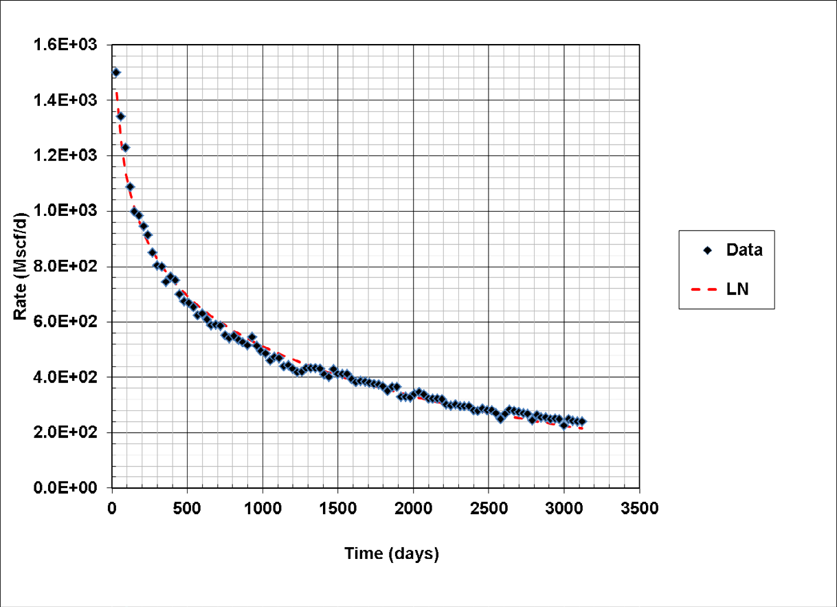
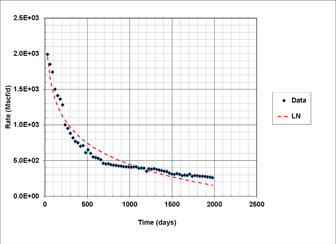
The logarithm model LNDM was applied to four major North American shale gas fields: Barnett, Fayetteville, Haynesville, and Woodford [7]. Figures 1 and 2 present the regression fit of the LNDM model to shale gas production type curve for the Barnett and Woodford shales respectively [8]. The LNDM model parameters from linear regression are given in Table 3. Rates expressed in Mscf/d define the units of and a λ as Mscf/d and day respectively.
| Shale | Constant | Flow Regime Examples |
|---|---|---|
| Barnett | a b λ | -261.1 2315.8 0.000141 |
| Woodford | a b λ | -430.17 3419.0 0.000353 |
Table 2: LNDM Parameters for Shale Gas Examples.
The fit of the LNDM model to the Barnett shale gas production type curve is a reasonable fit, while the fit of the LNDM model to the Woodford shale gas production type curve is not as good a fit. It is reasonable to expect that the LNDM model may not be suitable for all applications.
Application of the Logarithm Model to Shale Oil Production
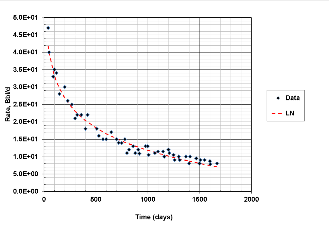
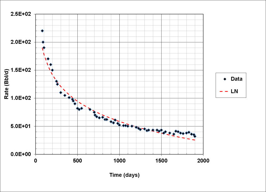
Figures 3 and 4 present the regression fit of the LNDM model to shale oil production data for the Eagle Ford and Bakken shales respectively [8]. Applications of the hyperbolic decline curve model and a stretched exponential decline curve model to shale oil production data are illustrated in Fanchi [9]. The LNDM model parameters from linear regression are given in Table 4. Rates expressed in Bbl/d define the units of and a λ as Bbl/d and day respectively.
| Shale | Constant | Flow Regime Examples |
|---|---|---|
| Bakken | a b λ | -51.785 416.32 0.000323 |
| Eagle Ford | a b λ | -9.3114 76.185 0.000280 |
Table 3: LNDM Parameters for Shale Oil Examples.
The fit of the LNDM model to the Eagle Ford shale oil production type curve is reasonable. The fit of the Bakken shale oil production type curve may be considered a reasonable representation, but another decline curve model might provide a better fit of the nonlinearity of the type curve.
Conclusions
A decline curve analysis model called the logarithm model (LNDM) was developed for flow rate proportional to the logarithm of time. The functional relationship between flow rate and logarithm of time was inferred from a study of flow regimes. We show how to use the rate-time relationship to calculate cumulative production at a specified economic limit for the LNDM model.
The use of the logarithm of time requires a careful interpretation of volumetric flow rate at the initial condition. The initial condition for the LNDM model states that the initial flow rate is the volume of production during the first period of time divided by the first period of time.
The LNDM model was illustrated by applying it to shale gas production and shale oil production decline curves. The decline curves represent a selection of North American shales.
References
-
Arps JJ (1945) Analysis of Decline Curves. Trans 160(1): 228-247.
-
Lee J (2007) Fluid Flow Through Permeable Media, Section 5 Diagnostic Plot. In: Lake LW (Ed.), Petroleum Engineering Handbook. Volume V, Reservoir Engineering and Petrophysics, Society of Petroleum Engineers, Richardson, TX, pp: 719-894.
-
Sun H (2015) Advanced Production Decline Analysis and Application. Petroleum Industry Press, Elsevier, Waltham, Massachusetts.
-
Fanchi JR, Christiansen RL (2016) Introduction to Petroleum Engineering, Wiley, Hoboken, New Jersey.
-
Ezekwe W (2020) Reservoir Engineering of Conventional and Unconventional Petroleum Resources. Tiga Petroleum, Houston, TX.
-
Panja P, Wood DA (2022) Production decline curve analysis and reserves forecasting for conventional and unconventional gas reservoirs. In: Wood DA, Cai J (Eds.), Sustainable Natural Gas Reservoir and Production Engineering. Volume 1, pp: 183-215.
-
Fanchi JR, Cooksey MJ, Lehman KM, Smith A, Fanchi AC, et al. (2013) Probabilistic Decline Curve Analysis of Barnett, Fayetteville, Haynesville, and Woodford Gas Shales. Journal of Petroleum Science and Engineering 109: 308-311.
-
Dutta R, Meyet M, Burns C, Van Cauter F (2014) Comparison of Empirical and Analytical Methods for Production Forecasting in Unconventional Reservoirs: Lessons from North America. SPE/EAGE European Unconventional Resources Conference and Exhibition, Society of Petroleum Engineers, Vienna, Austria.
-
Fanchi JR (2020) Decline Curve Analysis of Shale Oil Production Using a Constrained Monte Carlo Technique. Journal of Basic & Applied Sciences 16: 61-67.
- Nigeria’s Vulnerability in the Face of Global Energy Policy
- A Simulation Study of Investigation of Optimum Oil Production Performance by Applying Various Gas Injection Methods in Oil Reservoir
- Characterization of Permo-Triassic Reservoirs through Thermal Maturity Assessment of Westphalian Source Rocks in the Cheshire Basin
- Influence of Microwax on the Rheological and Thermal Behaviour of a Wax Crude Oil
- Real-Time Monitoring and Performance Optimization of Steam Injection in Heavy Oil Reservoirs Using Fiber Optic Sensing and Integrated Predictive Simulation Models
- Rapid On-Site Determination of the Total Petroleum Hydrocarbon Content of Soils by Handheld Fourier Transform Near-Infrared Spectroscopy: Development of a Global, Site- and Scanner- Independent Calibration Model