Thermal Simulations of Gas Lift and Water Injection Wells for Magurele Field Development: Future Strategies
A secondary recovery techniques are those used after natural energy depletion of an oil or a gas reservoir to boost its production such as gas lift and water injection. Both methods have been proved their success and effectiveness for enhancing field production. However, each reservoir or field has its own criteria and they may be ineffective depending field criteria and future plans. Furthermore, a field development strategy is considered as a key activity for enhancing the field recovery. Therefore, the aim of this article is to do well thermal simulation and analysis during making gas lift and water injection for Magurele field development at different conditions such temperature, tubing size, and production parameters. Several strategies are suggested from putting a new drilled well (M#206) on production till abandonment. A sensitivity study is done to know the effect geothermal zones and tubing size on well performance and flow regimes. It was found that utilizing a reservoir temperature of 70°C and tubing 3 1/2, all production activities displayed normal fluid and wellbore temperature profiles, using larger tubing or producing from the high temperature (HT) zone has only a minimal impact on the pressure profile, only slightly increasing surface pressures and The suggested production activities are unaffected by the higher temperature. With regard to the flow regime created by strategies, starting usage circumstances for tubing 3 1/2", with the exception of injection, which is turbulent in all scenarios, the flow regime is slug flow between 70°C and HT zones. Additionally, it seems like the bubbly flow is at shallower depths. Due to the use of 4 1/2-inch, the flow regime is altered to transitional and bubbly flows at deeper depths. This study helps to maximize the reservoir output and keep the new drilled wells usable and useful as long as possible.
Introduction
Not only do gas and oil have differing physical properties, but gas and oil production also differs for strictly economic reasons. A gas reservoir is always directly connected to a market via a pipeline; as a result, the physical characteristics of the reservoir cannot always determine the best depletion way because the market must be able to accept the gas. Production from an oil field can be according to an optimal development and depletion trend, based on its own merits. Therefore, the production and marketing stages have a close link for an oil field. The oil field may be developed gradually, which is another significant distinction. Early in the field’s development, oil production starts, providing further details on the oil reservoir. After the field starts to produce, some years later, the best field development strategy is chosen, and this choice is then based on a thorough understanding of the reservoir. The gas sales contract must be executed before gas production from the field can start. Before field development gets started, the fundamental variables needed to identify the field’s ideal development strategy must be known. It is therefore impossible to get comprehensive information about these characteristics. As a result, there are a lot of unknowns when planning the field developmental process in conjunction with an oil storage and a gas sales contract. The creation of an ideal development strategy for any field is constantly influenced by the usual traits of the producing field and the market that the field will service. Prior to designing the field’s development plan, which is actually dependent on the oil storage tanks and its marketing, and the gas-sales contract that must be reached in order to commit the natural gas reserves to the market, one must have a solid understanding of the field’s parameters, such as the total amount of reserves, the productivity of the wells, and the dependence of production rates on pipeline pressure and reserve depletion. The estimation of delivery rates from a collection of wells or a field to a point of sale or transfer is one of a fluid supply engineer’s major concerns. At this location on the main pipeline, the fluid must arrive at certain conditions. The flow through the reservoir(s), flow through the production strings of the wells, flow through the field gathering system and processing equipment, compression of the gas, and, finally, flow through an auxiliary pipeline to the point of sale and/or transfer are all required components of the overall production system [1, 2].
Artificial lift techniques and water injection are the secondary recovery methods that enhance the field production. Furthermore, they are considered part of the field development process after primary depletion [3, 4, 5, 6]. With gas lifted output levels above 1 million bopd, gas lift is the most used type of artificial lift. This accounts for almost 70% of the entire production group that was fraudulently increased [4]. Undoubtedly, field development planning and production operations depend heavily on the design and functioning of gas lift systems. Therefore, the gas lift and water injection are keys activity in developing the oil and gas field.
Consequently, the aim of this article is to do well thermal analysis during making gas lift and water injection for Magurele field development with different conditions such temperature, tubing size, and production parameters. In order to do this study, it is necessary to review the basic theories and mathematics included in this study such as heat transfer, multiphase flow, gas lift, water injection, development patterns, and field development strategies.
Well Heat Transfer
Heat is transmitted to and from rock throughout different well operations. Significant cooling occurs during water injection procedures, which has been shown to assist fracturing or pressure maintenance operations. Heat is also transmitted to the surface while normal drilling or production [7]. Furthermore, thermal responses include [7]:
- Temperatures in the casing and tubing strings and risers
- Temperatures in the annuli between the strings
- Temperature of the formation
- Different flow streams’ pressures
- Uncemented annuli pressure changes
Heat transfer in a wellbore is a well-established field, with defined methods for calculating temperatures in wells. It is vital to know the temperatures in the wellbore throughout production, injection, drilling, and shut-in from the standpoint of casing design and analysis. Cementing temperatures are normally produced by a particular circulation case followed by shut-in [7]. The heat transmission in the borehole during production or injection operation through tubing was explored in an early work on the wellbore temperatures by Ramey [8], while the heat transfer during circulation and drilling operations was examined by Raymond [9]. The publications by Ramey [8] and Raymond [9] are important because they present the fundamental physics of the wellbore heat transport. Hasan and Kabir [10] provide a detailed overview of all aspects of the wellbore heat transmission as well as a bibliography of significant publications from the previous several decades. To show the historical sequence of thermal modeling, studies and simulation; table published by Ivan, et al. [11] shows a background of the previous research studies and approaches.
The wellbore simulator solves the energy equation for the wellbore and formation and solves the equations shown below of mass, momentum, and energy conservation for each flow stream.
$$m = \rho v A = \text{constant}$$
$$\Delta P = \rho v \Delta v + \int_{\Delta z} \rho g \cos \phi dz \pm \int_{\Delta z} \frac{2 f \rho v^2}{D_h} dz = 0$$
$$\int_{\Delta z} \rho \varepsilon A dz = -\int_{\Delta z} P \frac{dv}{dz} Adz + \Phi + Q + R$$
$$\rho_1 C \frac{\partial T}{\partial t} = \frac{1}{r} \frac{\partial}{\partial t} \left( r K_z \frac{\partial T}{\partial t} \right) + \frac{\partial}{\partial z} \left( K_z \frac{\partial T}{\partial z} \right) + q \gg \text{formation Heat Transfer}$$
More details about solving the above equations in 1, 2 and 3 dimensions are fully discussed and expressed by Aadnooy, et al. [7].
Concepts of Multiphase Flow
The flow behavior is far more complicated for multiphase flow in pipes than it is for single phase flow. Differences in density often cause the phases to split. Due to the varying densities and viscosities of each phase, shear forces at the pipe wall are different for each phase. The in-situ volumetric flow rate of the gas is increased by the highly compressible gas phase expanding with a decrease in pressure. As a result, the gas and liquid phases often move through the pipe at different speeds. Slippage occurs in upward flow because the less dense, more compressible, and less viscous gas phase tends to flow at a higher velocity than the liquid phase. The liquid, however, frequently moves more quickly than the gas in downward flow [12]. The basic ideas for the flow parameters particular to multiphase flow in pipes are introduced and discussed in this section. The description of flow patterns includes information on tools for predicting their occurrence. The benefits and drawbacks of using empirical correlations based on dimensional analysis and dynamic similarity are discussed. To shortly describe the mathematical calculations of the included parameters in multiphase flow, the following expressions and equations have previously been presented by Brill and Mukherjee [12]:
$$q_0 = q_{0_w} B_0$$
$$q_w = q_{w_w} B_w$$
$$q_g = \left( q_{g_w} - q_{0_w} R_s - q_{w_w} R_{sw} \right) B_g$$
$$B_g = p_{sc} ZT / p Z_{sc} T_{sc}$$
$$q_L = \frac{w_i \left( 1 - x_g \right)}{\rho_L}$$
$$q_g = w_i x_g / \rho_g$$
$$x_g = \frac{VM_g}{VM_g + VM_L}$$
$$\lambda_L = \frac{q_L}{q_L + q_{lg}}$$
$$f_0 = \frac{q_0}{q_0 + q_w}$$
$$v_{SL} = q_L / A_p$$
$$v_{SG} = q_g / A_p$$
$$v_m = \frac{q_L + q_g}{A_p} = v_{SL} + v_{SG}$$
$$v_L = v_{SL} / H_L$$
$$v_g = \frac{v_{SG}}{1 - H_L}$$
$$v_s = v_g - v_L$$
$$\rho_L = \rho_a f_0 + \rho_w f_w$$
$$\sigma_L = \sigma_0 f_0 + \sigma_w f_w$$
$$\mu_L = \mu_0 f_0 + \mu_w f_w$$
$$\mu_s = \mu_L H_L + \mu_g \left( 1 - H_L \right)$$
$$\mu_s = \left( \mu_L H_L \right) \times \left[ \mu_g \left( 1 - H_L \right) \right]$$
$$\mu_w = \mu_L \lambda_L + \mu_g \left( 1 - \lambda_L \right)$$
$$\rho_s = \rho_L H_L + \rho_g \left( 1 - H_L \right)$$
$$\rho_n = \rho_L \lambda_L + \rho_g \left( 1 - \lambda_L \right)$$
$$\rho_k = \rho_L \lambda_L^2 + \rho_g \left( 1 - \lambda_L \right)^2$$
$$h = h_L \left( 1 - x_g \right) + h_g x_g$$
$$\frac{dp}{dL} = \frac{f \rho_f v_f^2}{2d} + \rho_f g \sin \theta + \rho_f v_f \frac{dv_f}{dL}$$
$$\left( \frac{dp}{dZ} \right)_t = \left( \frac{dp}{dZ} \right)_f + \left( \frac{dp}{dZ} \right)_el + \left( \frac{dp}{dZ} \right)_acc$$
$$\Delta p = \int_0^L \left( \frac{dp}{dL} \right) dL$$
For more details, Brill and Mukherjee [12] discussed totally theories and all equations of multiphase flow. Various correlations, their conditions and applicability were also explained.
Flow Assurance Modeling
Typically, flow assurance analysis is needed to complete the oil and gas development project. This analysis consists of: stable line sizing and transient assessment for production of gas, gas condensate, volatile crude oil, black oil fields, heavy/viscous crude oil, and tar sands; dimensioning of the stable line and transient analysis for the case of gas or water reinjection; dimensioning of the stable line for the production chemical distribution system; and optimization. A sophisticated integrated system, which incorporates reservoir characterization, PVT fluid characterization, and material properties, is what underpins flow assurance modeling. A sophisticated integrated system, which incorporates reservoir characterization, PVT fluid characterization, and material properties, is what underpins flow assurance modeling. Typically used as the foundation for flow assurance design and analysis, flow assurance requirements allow for the formulation of a strategy to address flow-specific impediments and difficulties (Figure 1). These needs include fluid production flow rate anticipated, fluid characterization, and environmental characteristics [13].
![Figure 1: Phase diagram for different flow assurance problems [13].](/fulltextimages/9244/fig_1.png)
To know steps of the flow assurance, the following procedures and phases are followed while flow assurance modeling [13]: 1. Analog fluids are necessary to determine properties like density 10° API, viscosity at reservoir temperature 10 cP, temperature for wax 20°C, rock and consolidation materials, limited understanding of porosity, permeability, presence and resistance of the aquifer, water composition, GOR, hydrate, asphaltene, etc. during the selection of a field for exploration. At this time, there are no sufficient flow assurance works. However, the very minimum amount of effort required is to calculate the hydrate curve based on the GOR composition, scale trend based on analog water composition, wax appearance temperature based on analog fluid, and asphalt variation trend based on analog fluid. 2. It is an opportunity to assess reservoir pressure, saturation pressure, GOR, density, viscosity, AOP, WAT, and SARA when the first well is explored and the first fluids are accessible. The assessment of the aquifer’s resistance to pressure, compartmentalizing the reservoir, figuring out the water’s composition, setting the pressure at the start of the process, estimating the GOR, estimating the hydration conditions, porosity, permeability, etc. will all come next. A steady state flow instrument is used for line size and initial routing in flow assurance investigations at this level.
3. Fluids (including secondary fluids) are accessible for testing after the flow test is implemented and the well evaluation is attached. The ability of doing a drill rod test is also an option. Conditions are favorable for obtaining information on water composition, reservoir compartmentation, and a sizeable sample of crude oil to assess hydrate clogging and asphalt deposition. The examination of concepts, update of line sizing utilizing multiphase flow models for transient analysis, location of wells, layout of flow lines, and rock consolidation, as well as the creation of various concepts with transient analyses are all examined in appropriate debt assurance studies (increase-based start, stop for recharge, exhaust separator sizing, slugging separator sizing). 4. Concept choice. Initially, a choice of operating system, such as an FPSO, semi-submersible, spar, artificial island, etc., is made based on national dangers. The timing of water injection, gas separation, additional fluid recovery vs capex and opex, etc. are other considerations that need to be taken. Flow assurance involves assessing technical options, resolving particular issues, and calculating the maximum rates of erosion in the flow lines for gas ascent. The formulation of operating procedures will also be aided by network flow analysis utilizing the flow model for steady-state flow rates or transient multiphase flow simulators for start-up and shut-down transient sequences.
| Geometry | Study/Model | Conditions | |
|---|---|---|---|
| Poettmann-Carpenter [14] | Vertical | Empirical | |
| Beggs-Brill [15] | Inclined | Empirical | |
| Baxendell-Thomas [16] | Vertical | Empirical | |
| Duns-Ross [17] | Vertical | Empirical | |
| Hagedorn-Brown [18] | Vertical | Empirical | Small Diameter |
| Mukherjee-Brill [19] | Inclined | Empirical | |
| Gray [20] | Vertical | Empirical | |
| Asheim [21] | Vertical | Empirical | |
| Orkiszewski [22] | Vertical | Empirical | |
| Chierici, et al. [23] | |||
| Dukler [24] | Vertical | Mechanistic | Holdup model issues |
| Aziz [25] | Vertical | Mechanistic | |
| Hasan and Kabir [26,27] | Vertical/ Inclined | Mechanistic | Wide range of tube sizes, crude gravity, GLR and W.C. |
| Ansari, et al. [28] | Vertical | Mechanistic |
Table 1: Flow Correlations in Pipes.
Flow Modeling Correlations
Several correlations have been developed and derived over the years using different data sets in order to more accurately predict the liquid content and pressure drop in a mobile fluid system. Today, most flow modeling is implemented using commercial software. Different flux correlations are reviewed and discussed in the literature Mukherjee H, et al. [19]. To review some of these correlations, in Table 1 we have presented the correlations and their typical application for flow through cylindrical pipes. Although each correlation was fit to the best accuracy of the data available at that time, extended applications of two- phase flow correlations can give an accuracy of ±50% in the flow system with various conditions [13].
Multiphase Flow Pressure Drop and Liquid Holdup: Vertical Horizontal
A basic summary of the multiphase flow relationship is provided and presented by Fancher, et al. [29] and Hetsroni [30]. They present the equations for single- phase flow, two-phase flow, particle flow, particle interface interaction, liquid film condensation, drag reduction, and measurement techniques. A good illustration of closure relations is discussed by Roullier, et al. [31]. A description of the general multiphase flow simulator is given in detail by Jansen [32]. CV for multiphase (vertical well) flow pressure drop correlations is discussed in detail by Brill and Mukherjee [19]. Today, many of these correlations are still in use. Different flow regimes have been identified and explained in recent decades. These are shown in Figure 2 for horizontal and vertical flow. At equilibrium, liquid holdup does not change with respect to vertical or horizontal flow over long lengths. However, local retention can change in the case of slug or churn flow [13]. Several correlations have been developed to determine liquid trapping in vertical or horizontal configuration, such as Turner, et al. [33], Hinze [34], Coleman, et al. [35] and Child and Brauer [36].
![Figure 2: Plots of multiphase flow regimes [13,37].](/fulltextimages/9244/fig_2.png)
Field Development Pattern
Recovery from such a field is conceivable up to a predetermined pressure of abandonment. This is the lowest pressure at which wells can continue to produce fluids at a pace high enough to pay for operations. The final economic recovery, which in the case of gas can reach to 80 and 90% of the gas in place, is determined by the point at which the line indicating the abandonment pressure crosses the depletion line. By choosing a drilling and production plan, the issue of actually producing the oil or gas in the formation in the most cost-effective manner is resolved. How many wells are required, when should they be drilled, and how much output from each well should be some of the problems that need to be addressed? Several production tests must be run on the first finding well in order to evaluate this. Later tests conducted in the appraisal wells will add to the results of these tests. A significant indicator of when a reservoir has to be developed is the normal productive life cycle of the reservoir. The basin has been identified at this time, but before fluids production can start, a system for gathering fluids from the field and transporting them by pipeline must be ready. The petroleum field’s production schedule should be set up so that the market can absorb the generated fluids, such as those from gas distribution systems, oil refineries, and oil storage facilities. The pace at which production may be increased as a result of this will often be constrained. On the other side, drilling schedules, processing, and transportation facilities may put a cap on the rate of production buildup. The production timeline for the field may also be influenced by economic factors. Consider a production plan in which there are three distinct phases: (1) a time of production growth; (2) a phase of constant rate output; and (3) a phase of production decrease. Reservoir deliverability graphs for various tubing head pressures may be used to determine the field development timetable. Here, we would simulate two patterns of field development plans [1, 2, 3, 4, 5, 6].
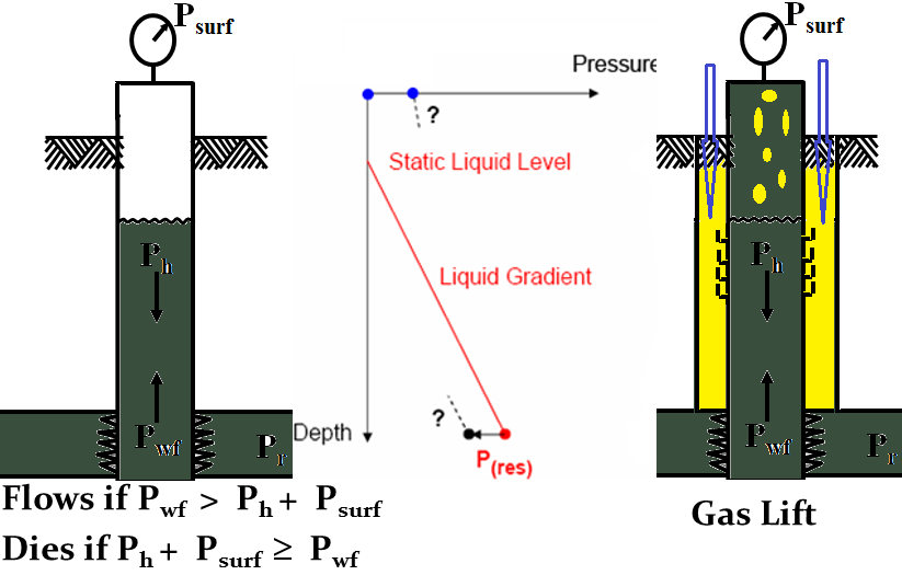
Gas Lift
Gas lift is an artificial lift technique that boosts formation gas with high-pressure gas from an external source to elevate the well fluids. According to the gas lift concept, injecting gas into the tube causes the fluids to become less dense while the resulting bubbles “scrubbing” the liquids. Both elements work to reduce the flowing bottom hole pressure at the tubing’s shoe (Figure 3). Today, continuous and intermittent flow are the two fundamental forms of gas lift. Each strategy, along with its design, benefits and drawbacks, is briefly described by [3, 4, 5, 6, 37].
Regarding our simulation using wellcat software, the surface injection pressure used to activate the gas lift is the pressure input in this situation. It is only used to compute the annulus fluid characteristics needed to calculate heat transfer. It is not advised to spend much time obtaining a correct number for this input because it has a negligible impact on the computations’ outcomes. Most circumstances will be satisfied by the default setting. As an alternative, the following two-step iteration may be used to perform a more exact calculation [38]:
As an alternative, the following two-step iteration may be used to perform a more exact calculation as follows:
- Calculating the gas lift operation using the injection pressure’s default value. Take note of the pressure that results in the tube at the gas lift valve’s depth.
- Carrying out the computation once more, increasing the input injection pressure to the pressure computed in step one plus.
- The pressure decreases anticipated in the annulus from the surface to the gas valve’s depth as a result of friction.
- The pressure drop in the gas lift valve at the intended flow rate.
Water Injection
Waterflooding is a water injection technique for pressure maintenance to boost oil reservoir recovery. “Primary production” which employs the reservoir’s inherent energy to generate oil, is usually followed by “secondary recovery,” which uses water to boost oil recovery. An oil reservoir is often water flooded in order to boost oil output and, eventually, oil recovery. This is done through “voidage replacement,” which involves injecting water to raise the reservoir pressure to its starting level and keep it there. Water removes oil from the pore spaces, however the effectiveness of this removal relies on a variety of circumstances (e.g., oil viscosity and rock characteristics). Voidage replenishment has also been utilized in oil fields like Wilmington (California, US) and Ekofisk (North Sea) to reduce further surface subsidence [2, 37]. Petroleum industry and scientific societies have released several important and in-depth books on waterflooding technology during the past four decades, for example those that are written by Craig [39], Willhite [40], and Rose, et al. [41].
Magurele Field Description
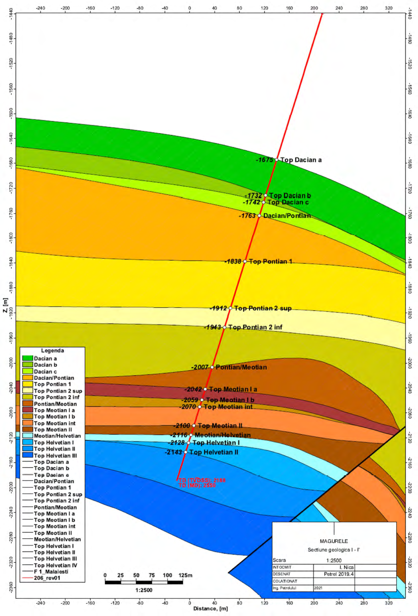
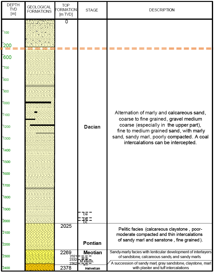
Magurele is an onshore commercial oil field that is considered as a part of structural alignment Malaiesti – Coada Calului – Magurele – Pacureti, located in Precarpatian Depression, Miopliocene subzone. Magurele structure contains accumulations of hydrocarbons in Helvetian, Meotian, and Dacian collectors. The cross sectional geological column is shown in Figure 4. Shortly, lithology description is addressed as following (Figure 5).
- Dacian is composed of an alternation of marly and calcareous sand, coarse to fine grained, gravel medium coarse (especially in the upper part), fine to medium grained sand, with marly sand, sandy marl, poorly compacted. A coal intercalations can be intercepted.
- Pontian is formed of Pelitic facies (calcareous claystone, poor-moderate compacted and thin intercalations of sandy marl and sanstone, fine grained).
- Meotian consists of sandy-marly facies with lenticular development of interlayers of sandstone, calcareous sands, and sandy marls.
- Helvetian is a succession of sandy marl, gray sandstone, claystone, marl with plaster and tuff intercalations.
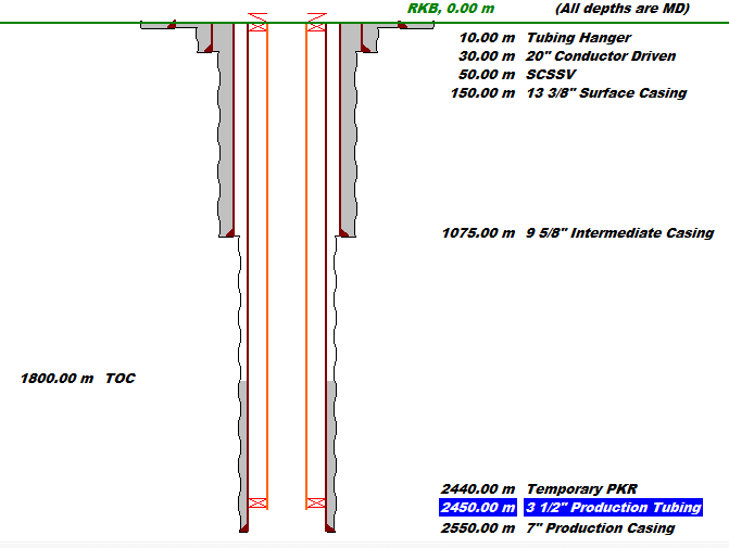
Well M#206 is located at Meoţian in block A and aims Meotian (M intermediate + M Ib). This well was drilled in 2022 as a produced oil well from this reservoir. The well was drilled directional: 2456 m TVD/2550 m MD with a displacement 627 m/360º. To assess the current state of reservoir wells were analyzed: 68 bis, 69, 76, 85 and 369 Magurele. In regard to the final depth (2456 m TVD) of maximum temperature well, an estimated value of 68-70° C. The reservoir pressure is 250 bar. Regarding this reservoir, all wells initially were naturally produced since 1977 and some of them were abandoned now. Our target here is to simulate two techniques of the secondary recovery which are suitable for recovery improvement and reservoir pressure maintenance.
Results and Discussions
First of all, the used software is called wellcat which is part of Landmark software developed by Halliburton Company and it a thermal tool for primary, secondary and some of tertiary recovery techniques. In this software, production simulations (prod module) are utilized to simulate heat transfer and fluid flow during production and workover operations. They can also be used for the following purposes [38]:
- Calculation of temporary well temperature and pressure during oil, gas, and / or water production
- Modeling gas lift operation
- Modeling spiral tubing operation
- Modeling water injection operation
- Impact of vacuum insulation Modeled tubing
- Prediction of shutdown temperature and pressure during circulation operation
- Hydraulic calculation during circulation operation
- Modeling of kill operation
- Modeling of squeeze cement activity
- Modeling of point cement plugging operation
- Well for pipe stress and buckling analysis
- Calculation of temperature and fluid pressure.
- Calculation of ring liquid temperature for use in ring liquid expansion calculation.
To simulate well performance thermally through natural flow, gas lift and water injection in the Magurele field so as to know if both techniques of the secondary recovery are effective or not, the previous strategies are suggested during putting a well M#206 on production till abandonment with the estimated parameters. Thermal simulation study and flow regime analysis are shown in Figures 7 through 9 and Tables 2 & 3 for completion string appeared in Figure 6 and reservoir data that are previously presented. It was found that all the production operations showed normally fluid and wellbore temperature profiles during using 70°C as an actual reservoir temperature, and tubing 3 1/2”/ 12.7lb/ft/ L-80 (Figures 7&8 a). Both profiles brought fluid and wellbore to a temperature between 60 and 80°C. However, the early gas lift reduces both profiles during using higher tubing size 4 1/2” and also has slightly impact on the other operations (Figures 7 & 8 b). Assuming having a geothermal zone or high temperature reservoir with 150°C the higher temperature has no impact on the behavior of the suggested production operations, only it brings wellbore and fluids to surface with higher temperatures between 70 and 110°C (Figures 7 & 8 c). Regarding the pressure profiles of various recovery and production strategies, they show a normal distribution with depth in all cases (Figure 9 a-c). Using higher tubing size or producing from HT zone has a little effect on pressure profile, only a slight increase of pressures at surface. Regarding flow regime formed during strategies, Tables 2 & 3 show the various types of flow regimes plotted in Figure 2 for natural flowing, gas lift and water injection. For initial conditions of using tubing 3 1/2”, 70°C and HT zones, the flow regime is slug flow for all cases except injection in which is turbulent at all. Furthermore, it appears the bubbly flow at lower depths. However, the type of regime is changed to transitional and bubbly flows at more depths with various meters due to using 4 1/2” tubing for production (Table 2). Turbulent flow remains for water injection as well.
Secondary, well M#206 was drilled as a natural produced oil well from Margurele field in 2022. However, taking a deep look to the offset wells; we noticed that most of these well are abandoned now after reservoir depletion. Thus, our study objective here is to set some strategies for future development plans in order to maximize the benefits from this well as possible as practical. Although some of reservoir and production well data are not available for us, this is not a big issue. These missing data will be estimated to do our simulations.
Regarding our suggested strategies for future plans, we use the following strategies from putting this well on production till its abandonment:
- Displacement to brine i.e the completion fluid which is CaCl2 with 10 ppg.
- Pulling the workstring, running the production tubing and set production packer.
- Initial production for well testing.
- Shut-in well for preparing permanent surface connection and manifold.
- Production for long time period with 100 bbl, and 60 bbl/day and 0.42 MMSCF/day for oil and water and gas respectively until reservoir pressure depletion to from 3625 to 2175 psi.
- Early gas lift at 1300 m and 2000 psi injection pressure for one year.
- Mid gas lift at 1600 m and 3000 psi injection pressure for one year.
- Late gas lift at 1900 m and 3500 psi injection pressure for one year
9. Water injection well with 50 gpm and 3000 psi injection pressure for two years.
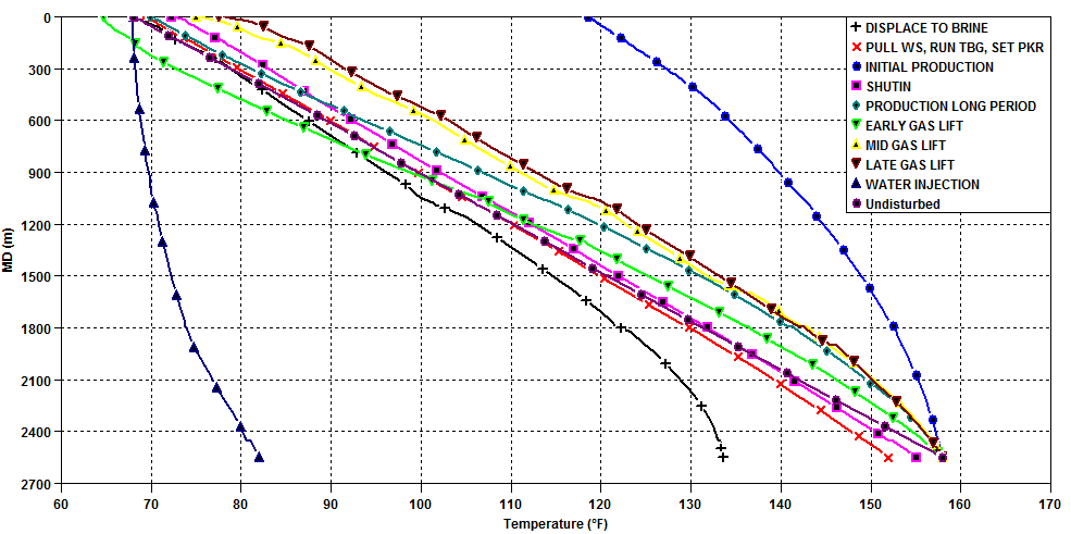
Figure 7a: Fluid temperature for various strategies; Temperature 70 oC, tubing 3 1/2”, L-80 and 12.7#.
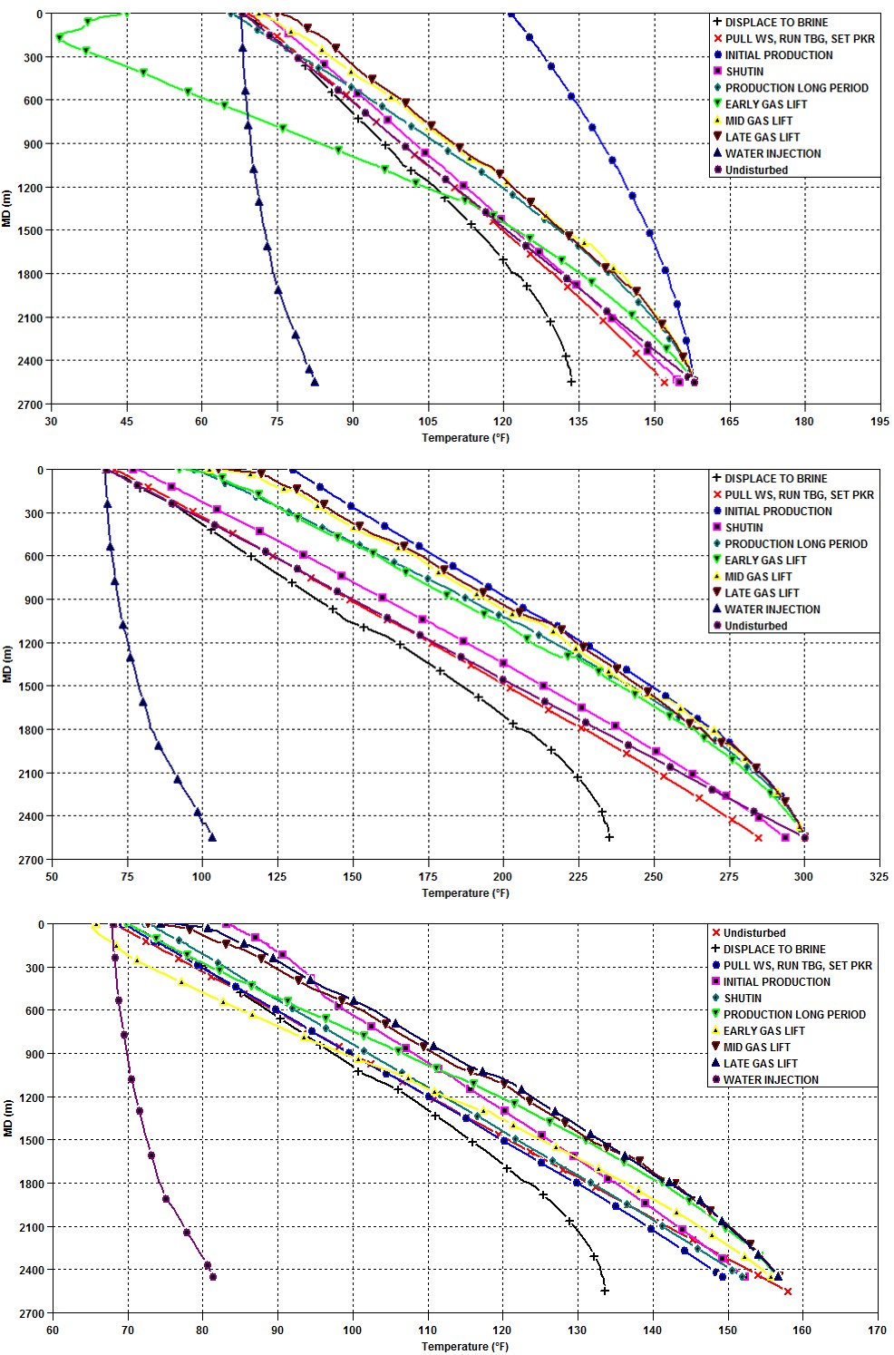
Figure 7b: Fluid temperature for various strategies; Temperature 70 oC, tubing 4 1/2”, L-80 and 12.7#.
Figure 7c: Fluid temperature for various strategies; Temperature 150 oC, 3 1/2” tubing.
Figure 8a: Wellbore temperature for various strategies; Temperature 70 oC, tubing 3 1/2”, L-80 and 12.7#.
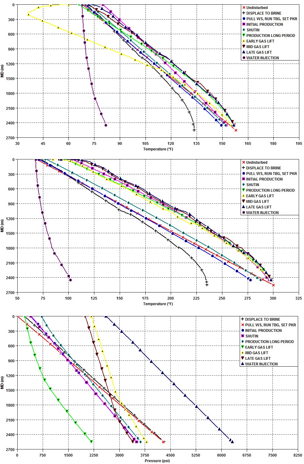
Figure 8b: Wellbore temperature for various strategies; Temperature 70°C, tubing 4 1/2”, L-80 and 12.7#.
Figure 8c: Wellbore temperature for various strategies; Temperature 150 oC, 3 1/2” tubing.
Figure 9a: Fluid pressure for various strategies; Temperature 70 oC, tubing 3 1/2”, L-80 and 12.7#.
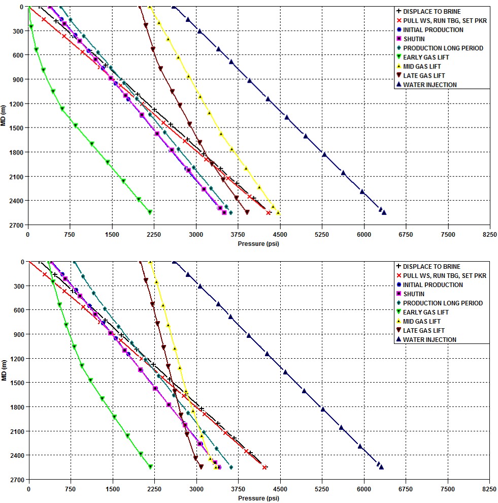
Figure 9b: Fluid pressure for various strategies; Temperature 70 oC, tubing 4 1/2”, L-80 and 12.7#.
Figure 9c: Fluid pressure for various strategies; Temperature 150 oC, 3 1/2” tubing.
| Natural Flow | Early GL | Mid GL | Late GL | Injection | |
|---|---|---|---|---|---|
| MD (m) | Flow Regime | Flow Regime | Flow Regime | Flow Regime | Flow Regime |
| 0 | Slug | Slug | Slug | Slug | Turbulent |
| 3.81 | Slug | Slug | Slug | Slug | Turbulent |
| 6.1 | Slug | Slug | Slug | Slug | Turbulent |
| 23.91 | Slug | Slug | Slug | Slug | Turbulent |
| 25.29 | Slug | Slug | Slug | Slug | Turbulent |
| 26.67 | Slug | Slug | Slug | Slug | Turbulent |
| 28.33 | Slug | Slug | Slug | Slug | Turbulent |
| 29.17 | Slug | Slug | Slug | Slug | Turbulent |
| 30 | Slug | Slug | Slug | Slug | Turbulent |
| 30.48 | Slug | Slug | Slug | Slug | Turbulent |
| 31.43 | Slug | Slug | Slug | Slug | Turbulent |
| 32.39 | Slug | Slug | Slug | Slug | Turbulent |
| 34.29 | Slug | Slug | Slug | Slug | Turbulent |
| 49.53 | Slug | Slug | Slug | Slug | Turbulent |
| 53.34 | Slug | Slug | Slug | Slug | Turbulent |
| 57.15 | Slug | Slug | Slug | Slug | Turbulent |
| 143.91 | Slug | Slug | Slug | Slug | Turbulent |
| 144.78 | Slug | Slug | Slug | Slug | Turbulent |
| 146.08 | Slug | Slug | Slug | Slug | Turbulent |
| 147.39 | Slug | Slug | Slug | Slug | Turbulent |
| 150 | Slug | Slug | Slug | Slug | Turbulent |
| 152.4 | Slug | Slug | Slug | Slug | Turbulent |
| 304.8 | Slug | Slug | Slug | Slug | Turbulent |
| 1075 | Slug | Slug | Slug | Slug | Turbulent |
| 1081.1 | Slug | Slug | Slug | Slug | Turbulent |
| 1796.95 | Slug | Slug | Bubble | Slug | Turbulent |
| 1800 | Slug | Slug | Bubble | Slug | Turbulent |
| 1803.05 | Slug | Slug | Bubble | Bubble | Turbulent |
| 2443.9 | Bubble | Slug | Bubble | Bubble | Turbulent |
| 2450 | Bubble | Slug | Bubble | Bubble | Turbulent |
| 2550 | Bubble | Bubble | Bubble | Bubble | Turbulent |
Table 2: Flow regimes for various strategies- 3/12” tubing for 70 and 150 oC.
| Natural Flow | Early GL | Mid GL | Late GL | Injection | |
|---|---|---|---|---|---|
| MD (m) | Flow Regime | Flow Regime | Flow Regime | Flow Regime | Flow Regime |
| 0 | Slug | Transitional | Bubble | Slug | Turbulent |
| 3.81 | Slug | Transitional | Bubble | Slug | Turbulent |
| 6.1 | Slug | Transitional | Bubble | Slug | Turbulent |
| 23.91 | Slug | Transitional | Bubble | Slug | Turbulent |
| 25.29 | Slug | Transitional | Bubble | Slug | Turbulent |
| 26.67 | Slug | Transitional | Bubble | Slug | Turbulent |
| 28.33 | Slug | Transitional | Bubble | Slug | Turbulent |
| 29.17 | Slug | Transitional | Bubble | Slug | Turbulent |
| 30 | Slug | Transitional | Bubble | Slug | Turbulent |
| 30.48 | Slug | Transitional | Bubble | Slug | Turbulent |
| 31.43 | Slug | Transitional | Bubble | Slug | Turbulent |
| 32.39 | Slug | Transitional | Bubble | Slug | Turbulent |
| 34.29 | Slug | Transitional | Bubble | Slug | Turbulent |
| 49.53 | Slug | Transitional | Bubble | Slug | Turbulent |
| 53.34 | Slug | Transitional | Bubble | Slug | Turbulent |
| 57.15 | Slug | Transitional | Bubble | Slug | Turbulent |
| 143.91 | Slug | Slug | Bubble | Slug | Turbulent |
| 144.78 | Slug | Slug | Bubble | Slug | Turbulent |
| 146.08 | Slug | Slug | Bubble | Slug | Turbulent |
| 147.39 | Slug | Slug | Bubble | Slug | Turbulent |
| 150 | Slug | Slug | Bubble | Slug | Turbulent |
| 152.4 | Slug | Slug | Bubble | Slug | Turbulent |
| 304.8 | Slug | Slug | Bubble | Bubble | Turbulent |
| 1075 | Bubble | Slug | Bubble | Bubble | Turbulent |
| 1081.1 | Bubble | Slug | Bubble | Bubble | Turbulent |
| 1796.95 | Bubble | Bubble | Bubble | Bubble | Turbulent |
| 1800 | Bubble | Bubble | Bubble | Bubble | Turbulent |
| 1803.05 | Bubble | Bubble | Bubble | Bubble | Turbulent |
| 2443.9 | Bubble | Bubble | Bubble | Bubble | Turbulent |
| 2450 | Bubble | Bubble | Bubble | Bubble | Turbulent |
| 2550 | Bubble | Bubble | Bubble | Bubble | Turbulent |
Table 3: Flow regimes for various strategies- 4/12” tubing and 70°C.
Conclusions
Good practical strategies are keys activity in Magurele field development such taking the appropriate decision at the suitable time for starting another technique of production enhancement. Thermal simulation study and flow regime analysis are performed to show well performance for a certain period (5 years after reservoir depletion with no flow naturally). This helps to keep the well M#206 flowing with a reasonable quantity of oil and gas. As conclusions, the temperature has insignificant effect on gas lift and water injection operations. Furthermore, various flow regimes appeared need a big attention to the surface producing and processing units. Any changes can be introduced to the model to show their impact on production. Finally, simulations and analysis of various condition with various strategies would help to boost well production and keep it flowing.
References
-
Ikoku CU (1992) Natural Gas Reservoir Engineering. Krieger Publishing Company.
-
Ahmed T (2010) Reservoir engineering handbook. 4th (Edn.), Gulf Professional Publishing, pp: 1472.
-
Report EP 93-2702 (1993) Artificial lift manual part 2A. Shell International Petroleum Maatschappij BV, The Hague, Exploration & Production.
-
EP 93-0235 (1992) Group Artificial Lift Statistics.
-
Brown KE (1984) The Technology of Artificial Lift Methods. Volume 2A, Penn-Well Books, Tulsa.
-
Neely AB, Gipson FW, Capps B, Clegg JD, Wilson P, et al. (1981) Selection of Artificial Lift Method. SPE Annual Technical Conference and Exhibition, SPE 10337.
-
Aadnoy B, Cooper I, Miska S, Mitchell RF, Payne M (2009) Advanced drilling and well technology. SPE, pp: 888.
-
Ramey HJ (1962) Wellbore Heat Transmission. J Pet Technol 14(4): 427-435.
-
Raymond LR (1969) Temperature Distribution in a Circulating Drilling Fluid. J Pet Technol 21(3): 333-341.
-
Hasan AR, Kabir CS (2002) Fluid Flow and Heat Transfer in Wellbores. SPE, Texas, USA, pp: 175.
-
Ivan R, Halafawi M, Avram L (2022) Offset Wells Data Analysis and Thermal Simulations Improve the Performance of Drilling HPHT Well. Pet Petro Chem Eng J 6(1): 1-15.
-
Brill J, Mukherjee H (1999) Multiphase Flow in Wells. SPE, Richardson, Texas.
-
Makogon TY (2019) Handbook of multiphase flow assurance. 1st(Edn.), Gulf Professional Publishing, Elsevier.
-
Poettman FH, Carpenter PG (1952) The multiphase flow of gas, oil and water through vertical flow strings with application to the design of gas-lift installations. In: Drilling and Production Practice. American Petroleum Institute API-52, p: 257.
-
Beggs HD, Brill JP (1973) A Study of Two-Phase Flow in Inclined Pipes. J Pet Tech 25(5): 607-617.
-
Baxendell PB, Thomas R (1961) The Calculation of Pressure Gradient in High-Rate Flowing Wells. JPT 13(10): 1023-1028.
-
Duns H, Ros NCJ (1963) Vertical flow of gas and liquid mixtures in wells. Proceedings of 6th World Petroleum Congress, Frankfurt, pp: 451-456.
-
Hagedorn AR, Brown KE (1965) Experimental study of pressure gradients occurring during continuous two phase flow in small-diameter vertical conduits. J Pet Technol 17(4): 475-484.
-
Mukherjee H, Brill JP (1985) Pressure drop correlation for inclined two-phase flow. J Energy Resour Technol 107(4): 549-554.
-
User’s Manual for API14P (1978) SSCSV Sizing Computer Program. 2nd(Edn.), API Appendix B, pp: 38-41.
-
Asheim H (1986) MONA, An Accurate Two-Phase Well Flow Model Based on Phase Slippage. SPE Prod Eng 1(3): 221-230.
-
Orkiszewski J (1967) Predicting Two-Phase Pressure Drops in Vertical Pipe. J Pet Tech 19(6): 829-838.
-
Chierici GL, Ciucci GM, Sclocchi G (1974) Two-Phase Vertical Flow in Oil Wells_Prediction of Pressure Drop. J Pet Technol 26(8): 927-938.
-
Dukler AE, Wicks M, Cleveland RG (1964) Frictional pressure drop in two-phase flow: an approach through similarity analysis. AlChE J 10(1): 44-51.
-
Govier GW, Aziz K (1972) The Flow of Complex Mixtures in Pipes. Van Nostrand Reinhold Co., New York.
-
Hasan AR, Kabir CS (1998) A Study of Multiphase Flow Behavior in Vertical Wells. SPE Prod Eng 3(2): 263-272.
-
Hasan AR, Kabir CS (1988) Predicting Multiphase Flow Behavior in a Deviated Well. SPE Prod Eng 3(4): 474- 482.
-
Ansari AM, Sylvester ND, Shoham O, Brill JP (1994) A Comprehensive Mechanistic Model for Two-Phase Flow in Wellbores. SPE Prod & Fac 9(2): 143-151.
-
Fancher GH, Brown KE (1963) Prediction of Pressure Gradients for Multiphase Flow in Tubing. SPE J 3(1): 59- 69.
-
Hetsroni G (1982) Handbook of Multiphase Systems. Hemisphere Publishing Corporation, McGraw Hill Book Company.
-
Roullier D, Shippen M, Adames P, Pereyra E, Sarica C (2017) Identification of optimum closure relationships for a mechanistic model using a data set for low- liquid loading subsea pipeline. SPE Annual Technical Conference and Exhibition, San Antonio, Texas, USA.
-
Jeppe JM (2009) Evaluation of a flow simulator for multiphase pipelines. Master of Science Thesis, Norwegian University of Science and Technology, Norway, pp: 1-132.
-
Turner RG, Hubbard MG, Dukler AE (1969) Analysis and prediction of minimum flow rate for the continuous removal of liquids from gas wells. J Pet Tech 21(11): 1475-1482.
-
Hinze JO (1955) Fundamentals of the hydrodynamic mechanism of splitting in dispersion processes. AICHE J 1(3): 289-295.
-
Coleman SB, Clay HB, McCurdy DG, Norris LH (1991) A new look at predicting gas-well load up. J Pet Tech 43(3): 329-333.
-
Child H, Brauer P (2017) Comparing HZ Critical rate models against Marcellus field data. Gas well deliquification workshop, Denver.
-
Lorenz, Michael D, Lyons, Pilsga WC, Gary J (2016) Standard Handbook of Petroleum and Natural Gas Engineering. 3rd (Edn.), Gulf Professional Publishing.
-
Halliburton Landmark, Providing you with the Choice & Flexibility to Digitally Transform your E&P Operations.
-
Craig Jr FF (1971) The Reservoir Engineering Aspects of Waterflooding, Vol 3, SPE Monograph Series, Richardson, Texas.
-
Willhite GP (1986) Waterflooding. Vol 3, SPE Textbook Series, Richardson, Texas.
-
Rose SC, Buckwalter JF, Woodhall RJ (1989) The Design Engineering Aspects of Waterflooding. Vol 11, SPE Monograph Series, Richardson, Texas.
- Nigeria’s Vulnerability in the Face of Global Energy Policy
- A Simulation Study of Investigation of Optimum Oil Production Performance by Applying Various Gas Injection Methods in Oil Reservoir
- Characterization of Permo-Triassic Reservoirs through Thermal Maturity Assessment of Westphalian Source Rocks in the Cheshire Basin
- Influence of Microwax on the Rheological and Thermal Behaviour of a Wax Crude Oil
- Real-Time Monitoring and Performance Optimization of Steam Injection in Heavy Oil Reservoirs Using Fiber Optic Sensing and Integrated Predictive Simulation Models
- Rapid On-Site Determination of the Total Petroleum Hydrocarbon Content of Soils by Handheld Fourier Transform Near-Infrared Spectroscopy: Development of a Global, Site- and Scanner- Independent Calibration Model