Predictive Models for Oil in Place for Oil Rim Reservoirs in the Niger Delta Using Machine Learning Approach
One of the key factors that analysts consider when calculating the economics of oil field development is the amount of oil in place (OIP). Conventional methods used for its estimation have some features affecting their predictive capabilities and applications. In addition, Oil bidders have limited time to evaluate and rank reservoirs from complex and large reservoir data packages - which sometimes fees are paid for their access. In this study, data-driven machine learning models - artificial neural network (ANN), support vector regression (SVR) and multiple linear regression (MLR) were developed for quick estimation of OIP for oil rim reservoirs in the Niger Delta. The models were evaluated using statistical error tools, and the results showed reasonable predictions. The sensitivity analysis performed on the selected input parameters showed that areal extent has the greatest impact on the estimation of the OIP with 29.94 %, oil formation volume factor has 22.74 % impact, oil column thickness was 16.61 %, m-factor has 13.29 %, water saturation was 9.01 %, and lastly porosity has 8.38 %. Comparison with recovery factor surrogate models existing in open literature were also carried out. The newly developed models can be helpful for oil bidders in ranking and evaluation of oil rim reservoirs in the Niger Delta.
Introduction
One of the key factors that analysts consider when calculating the economics of oil field development is the amount of oil in place (OIP). The amount of oil in place is the most crucial criterion for reservoir engineers to quickly determine if the found region is valuable or not [1]. Estimation of OIP is a key factor in oil price regulation, together with oil production and total demand [2]. The Akata formation, the Agbada formation, and the Benin formation are the lithostratigraphic units responsible for the tertiary siliciclastic deposits of the Niger Delta. The majority of the Niger Delta’s oil and gas reserves are found in the Agbada formation (Paralic Cycles), which is composed of alternating sandstone and shale bedsets that are considered to depict the delta front, distributary channels, and the deltaic plain. The top half has more sandstone than the lower part, indicating the Niger delta’s steady seaward movement through geological time. The sediments are a sequence of sand and shale successions accumulated through several relative sea level changes. These sediments feature distinct coarsening- upward, fining-upward, blocky, and serrated gamma ray (GR)/spontaneous potential (SP) log profiles [3, 4].
There are a lot of oil reserves in the Niger Delta, however they cannot be fully exploited due to the presence of large number of oil rim reservoirs. Onukwuri, et al. [5] stated that oil rim reservoirs, oil thickness less than 100 ft, contain substantial amount of hydrocarbon due to their large lateral extent. For oil rim reservoirs in the Niger Delta, there are many different studies predominately on development and optimization of production. However, very few literature has been published on the estimation of oil in place. The precision in estimating the oil in place depends on the method used. Basically, there are two conventional methods used to estimate the OIP - volumetric and the material balance approaches. Furthermore, other methods such as; analogy, decline curve analysis and reservoir simulation approaches are commonly used. Few explanations of these traditional methods are provided as follows:
**Analogy Method**
This is the most basic estimating technique; it is based on a geologic analogy with a nearby producing area and is utilized for undrilled or sparsely drilled areas [6]. Gehman and White [7] explained that, in its most basic form, evaluation by analogy states that if untested region A has a geological appearance similar to that of proven producing area B, then it must contain a comparable amount of oil and gas. However, it is the least accurate of the methods [8]. Thus, it is advised to use the analogy method in combination with other techniques to ensure that the results make sense within geological frameworks.
**Volumetric Approach**
This is the most common approach used for oil in place estimation. It is an initial approach used after completion. As the name implies, the calculations used in this approach depend on the reservoir volume, which may be determined using maps and petrophysical information from drilled wells [9]. The volumetric equation for estimating oil in place is expressed in Equation (1):
$$OIP = \frac{7758\phi A h (1 - S_{wi})}{B_{oi}}$$
where, $\phi =$ porosity (fraction), $A =$ areal extent of the reservoir (acres), $h =$ reservoir thickness (ft), $S_{wi} =$ initial water saturation (fraction), and $B_{oi} =$ initial oil formation volume factor (bbl/stb).
Though the volumetric method is the most commonly used tool for the estimation of OIP, it is associated with inherent uncertainties as a result of some assumptions made and also when the reservoir data are yet to be sufficiently determined. Nwosu [10] stated that the volumetric estimation made on wells should be updated by intervals as additional production data become available. Hossain, et al. [11] mentioned that reservoir boundary is subject to large errors. Therefore, this method cannot provide the EUR (Expected Ultimate Recovery).
**Material Balance Method**
This is another technique used in the estimation of OIP. The general material balance equation for estimating OIP is given in Equation 2:
$$N = \frac{N_p \left[ B_o + \left( R_p - R_s \right) B_{ig} \right] - \left( W_e - W_p B_o \right) - G_{ij} B_{ij} - W_{ij} B_w}{(B_o - B_{oi}) + (R_s - R_i) B_{ig} + m B_{ig} - 1} + B_{oi} (1 + m) \left[ \frac{S_{wi} C_w + C_i}{1 - S_{wi}} \right] \text{ A/P}$$
where, $N =$ initial oil-in-place (stb), $N_p =$ cumulative oil produced (stb), $G_p =$ cumulative gas produced (scf), $W_p =$ cumulative water produced, $R_{si} =$ initial gas solubility (scf/stb), $B_{oi} =$ oil formation volume factor (bbl/stb), $B_{oi} =$ initial oil formation volume factor (bbl/stb), $\text{A/P} =$ change in reservoir pressure (psi), $R_s =$ gas solubility (scf/stb), $B_{oi} =$ initial gas formation volume factor (bbl/scf), $B_{oi} =$ gas formation volume factor (bbl/scf), $W_e =$ cumulative water influx (bbl), cumulative water injected (stb), $W_{ij} =$ cumulative gas injected (scf), $G_{ij} =$ ratio of initial gas cap gas reservoir volume to initial reservoir oil volume, (bbl/bbl), $C_w =$ water compressibility (psi$^{-1}$), $C_j =$ formation (rock) compressibility (psi$^{-1}$) and $water formation volume factor (bbl/stb).
According to Nwosu [10], to use the material balance technique, sufficient production and pressure data should be available. On the other hand, Omoniyi, et al. [12] mentioned that for material balance to be used to estimate the reserve, five percent of its volume must have been recovered. The material balance method is made to assume that the reservoir is a single tank or area with consistent rock characteristics and a constant pressure across the reservoir at any given time and development stage [13]. The primary weakness in the material balance method is that; it tends to over-estimate the reservoir regardless of the tact and experience of the estimator.
**Decline Curve Analysis**
This is a means of predicting future oil and gas well production based on past production history. This approach is used when most of the oil and gas have been produced and the field production rate is declining [14]. Based on well conditions, there are three types of decline curves namely: exponential, hyperbolic and harmonic decline (Table 1).
| Decline Type | Exponential | Hyperbolic | Harmonic |
|---|---|---|---|
| Rate-time relationship | q=q es t i | q=q(1+nDt)-1/n t i i | q=q(1+Dt)-1 t i i |
| Rate-cumulative relationship | q q N i t p D | q in N (q1n q1 n) p 1n D i t i | q q N i log i p D e q i t |
Table 1: Rate-time and rate-cumulative production relationships.
where, qt, production rate (STB/D) at time t; qi, initial production rate; Np, cumulative production (STB); D, decline rate (STB/D/year); n, hyperbolic exponent.
The exponential and hyperbolic decline are frequently used to describe reservoir performances. Downey [15] pointed out that decline curve analyses can underestimate oil reserves and production rates, and overestimate production performance. He also further reported that this technique relies on past data and therefore does not take into the possibility of geological changes.
Reservoir Simulation
As reported by Nasar, et al. [1], reservoir simulators represent the reservoir as a collection of interconnected tanks using material balance and fluid flow equations. In general, a development strategy and operational conditions are placed on the system. A good match between observed history and simulated performance is required for reliable outcomes [6]. Simulation techniques require substantial amount of performance data for history matching and prediction, and also requires long simulation duration. More also, Nasar, et al. [1] reported that the main challenge associated with this technique is building a reservoir model that can highly depict the real reservoir.
Brief Review of Application of Machine Learning in Petroleum Industry
With the recent advancement of technology, artificial intelligence has been applied in the petroleum industry. Machine learning has the ability to aid and improve traditional reservoir engineering techniques for a wide variety of reservoir engineering problems [22]. For example, ANN has mostly been utilized in various aspects of reservoir engineering, for instance, reservoir modeling and characterization [22, 23], reservoir properties prediction [24, 25, 26], prediction of permeability [27], drilling operations [28, 29]. Also, other machine learning approaches such as Fuzzy Logic, Support Vector Machines (SVM), Random Forest (RF), and Multiple Linear Regression (MLR) have been employed in reservoir engineering problems [30, 31, 32, 33, 34].
The basic principle of Artificial Neural Network is to approximate a function between the input vector to the output category y):
$$ \hat {y} = f ^ {*} (x) \tag {3} $$
The mapping between input and output is given by:
$$ \hat {y} = f ^ {*} (x, \theta) \tag {4} $$
where θ consists of a weight , and a bias . Note that θ is
learnt by iterating over a given data.
An Artificial Neural Network comprises at least three layers denoted input, hidden with neurons, and output. Each layer connects with other layers with the help of weights (. The network performance is solely based on the adjustment of weights between these layers. Hidden layers assigned with transfer function are usually ‘log-sigmoidal’ or ‘tan- sigmoidal’. The output layer is assigned with a ‘pure linear’ activation function [35]. The above explanation is expressed mathematically as:
$$ \hat {y} = \sigma \left(x ^ {T} w + b\right) \tag {5} $$
where, σ is the transfer function, usually log-sigmoidal or
tan-sigmoidal, and xT is the transpose of the input vector, x.
In a bid to employ new approach to improve oil in place estimation, machine learning techniques have been considered. This work therefore presents ANN, SVR and MLR model developments for predicting OIP for oil rim reservoirs in the Niger Delta.
Dataset Used for the Study
The oil rim dataset of more than 200 reservoirs in the Niger Delta, of which some have been reported by Obah, et al. [36] and Ukpong, et al. [37] and Omeke, et al [38] used for the development of the models in this study were obtained from different sources - well logs, well testing, seismic analysis, simulation studies, pressure buildup test, area versus depth plot obtained from mapping packages, reservoir isochores, proprietary software to estimate probabilistic in place volumes and reservoir engineering calculations where necessary. The statistical description of the data is presented in Table 2.
| Parameters | Min. Value | Max. Value | Mean | Standard Deviation | Variance |
|---|---|---|---|---|---|
| Oil column thickness (ft) | 1 | 100 | 54 | 22.85 | 522.07 |
| Porosity (%) | 15 | 35 | 26.1 | 4.08 | 16.62 |
| Water saturation (%) | 5 | 73 | 24.6 | 10.8 | 116.63 |
| Oil formation volume factor (rb/stb) | 1.08 | 6.27 | 1.47 | 273.4 | 74748.03 |
| Gas cap, m-factor | 0.01 | 4.73 | 0.66 | 0.8387 | 0.7 |
| Area (acres) | 19.66 | 64593.74 | 856.64 | 5131 | 26327160 |
| Average net pay (ft) | 0 | 524 | 58.53 | 47.92 | 2296.18 |
| Temperature (oF) | 125 | 240 | 175.2 | 25.39 | 644.8 |
| OUT pressure (psi) | 2148 | 5984 | 3717.4 | 715.06 | 511308.8 |
| OUT depth (ft) | 4930 | 13017 | 8486.15 | 1584.95 | 2512062 |
| Rsi (scf/bbl) | 76 | 6234 | 925.76 | 593.31 | 352021.2 |
| Permeability (md) | 3.36 | 18225 | 797.97 | 1439.87 | 2073213 |
| OIP (mmstb) | 0.9 | 158.4 | 21.3 | 24.988 | 624.4042 |
Table 2: Statistical description of oil rim dataset used in this study.
Models Development
Before the training and development of the models, pairplots in python seaborn library was carried out for the parameters in Table 2 to check their relationships, and patterns, with the expected target property – OIP to enable the selection of the input properties. However, there were no distinct trends between the features and the target parameter. So, based on the knowledge of the parameters in volumetric method and the importance of other parameters, six (6) input variables were considered, namely; porosity (%), oil column thickness (ft), areal extent (acres), oil formation volume factor (bbl/stb), gas cap size (m-factor), water saturation (%) to predict the (output) oil in place (MMSTB).
Development of the Artificial Neural Network Model
The ANN model was developed using the neural fitting tool box (nftool) of the Matrix Laboratory (R2015a MATLAB) mathematical software for the prediction of OIP. The input and output values were normalized to make the values suitable for training by the ANN algorithm using Equation 6.
$$ x _ {n o r m} = \frac {x _ {i} - x _ {m i n}}{x _ {m a x} - x _ {m i n}} \tag {6} $$ i min norm max min where denotes the normalized input or output variable, is the actual value to be normalized, and represents the minimum and maximum values of the actual parameter (value).
The normalized expressions for the input properties used for the development of the ANN model are presented through Equations 7 through 12.
$$ h _ {o _ {(n)}} = 0. 0 1 0 1 h _ {o} - 0. 0 1 0 1 \tag {7} $$
$$ B _ {o _ {(n)}} = 0. 1 9 2 6 B _ {o} - 0. 2 0 7 3 \tag {8} $$
$$ \varphi_ {(n)} = 5 \varphi - 0. 7 5 \tag {9} $$
$$ S _ {w _ {(n)}} = 1. 4 7 0 6 S _ {w} - 0. 0 7 3 5 \tag {10} $$
$$ A _ {(n)} = 2 E (- 0 5) A - 0. 0 0 0 3 \tag {11} $$
$$ m _ {(n)} = 0. 2 1 1 4 m - 0. 0 0 0 5 \tag {12} $$
are the normalized
values of oil column thickness, oil formation volume factor,
porosity, water saturation, area, and gas cap size, respectively.
The normalized dataset was split into 3 parts which are 70%,
15% and 15% for training data, test data and validation data
respectively. Following multiple trials of various network
topologies, the best network performance was found with
six input neurons, seven neurons in the hidden layer, and one
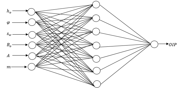
output neuron, resulting in the 6-7-1 network architecture.
Figure 1 shows the network topology of the newly developed
ANN model.
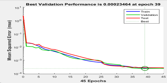
After several iterations, it was found that the network with seven hidden neurons had the best validation performance when the model was stopped at 39 epochs with an mean square error (MSE) of. The validation performance is shown in Figure 2. Summary of the parameter description for the developed ANN model is presented in Table 3.
| Parameters | Values |
|---|---|
| Training dataset | 174 (70% of the dataset) |
| Validation dataset | 37 (15% of the dataset) |
| Testing dataset | 37 (15% of the dataset) |
| Number of input neurons | 6 |
| Number of hidden layers | 1 |
| Number of neurons in the layer | 7 |
| Number of output neurons | 1 |
| Activation function (input layer) | Tansig |
| Activation function (output layer) | Purelin |
| Learning Algorithm | Levernberg-Marquardt |
| Number of epochs | 1000 |
| Target goal mean squared error | 105 |
| Architecture selection | Trial and Error |
Table 3: Parameter description of the developed ANN model.
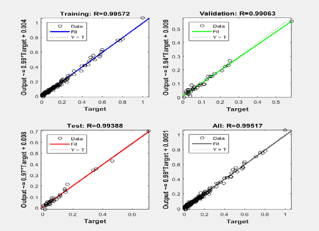
The performance efficiency of the developed model is presented in Figure 3, showing the scattered plot of the predicted oil in place versus the actual oil in place, in terms of training, testing and validation.
Thus the developed ANN model for predicting oil in place for oil rim reservoirs in the Niger Delta is given by Equation 13. This equation correlates the six input parameters (h,B_o,φ,S_wi,A,m) and the output, OIP.
() () () () () () ( )
• = + + + + + + × + ∑
6
1 1 n n n ANN o ij o ij ij w ij ij ij ij k n n n j OIP tansig h IW B IW IW S IW A IW m IW b LW b ϕ = (13) where the purelin and tansig are in-built MATLAB activation functions for the output and hidden layers; IW is the weight attached to the input neuron; LW is the weight attached to the hidden neurons and b1, bk are the biases in the hidden neuron and output layer neuron respectively. According to Agwu, et al. [28], the ‘tansig’ function is suitable for the application in the development of artificial neural network models because it performs operations in very fast approach when compared to other functions. Equation 14 expresses the correlation of the ‘tansig’ function.
2 (14) $$ T a n s i g = \frac {2}{\left[ 1 + E x p (- 2 n e t w o r k) - 1 \right]} $$ ( ) Thus, the values for the weights and biases of the developed model are presented in Table 4.
| IW 1 | IW 2 | IW 3 | IW 4 | IW 5 | IW 6 | b1 | LW | b k |
|---|---|---|---|---|---|---|---|---|
| 0.685801 | 0.755557 | -0.61782 | 0.146391 | 1.598598 | 0.985223 | -2.55987 | 1.97521 | -1.96732 |
| 0.606326 | -1.31617 | 0.221929 | -0.73283 | 0.587082 | -0.21037 | -2.02872 | -7.40073 | |
| 0.607569 | 0.962716 | 0.035803 | 0.303653 | -3.88356 | -0.01166 | -0.39921 | 6.771898 | |
| -1.02284 | -0.86053 | 0.921702 | 0.431266 | -0.14791 | 1.12337 | 1.075169 | 0.399309 | |
| 0.779506 | 1.564678 | -0.78411 | -0.42265 | 0.809694 | -1.18806 | -0.01725 | 0.391533 | |
| -0.5599 | 1.261749 | -0.19332 | 0.65746 | -5.71381 | 0.19068 | -3.10335 | -9.44174 | |
| -0.5599 | -0.70034 | -0.29039 | 0.2471 | 0.138854 | 0.405154 | -2.66434 | 1.811358 |
Table 4: Weights and biases of the developed ANN model.
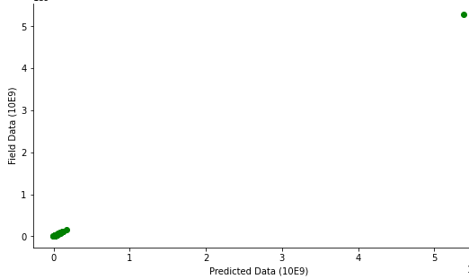
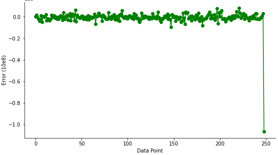
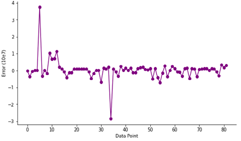
To evaluate the performance of the developed model, the comparison between field data and the predicted data is shown in Figure 4, while Figure 5 shows the error plots.
Development of the Support Vector Regression
For the SVR model, Jupyter notebook of the Anaconda software was employed using different libraries of python language for the prediction of oil in place. The scikit- learn module was mainly used, the pandas library and the matplotlib module was imported to the Jupyter notebook using the ‘import’ function. The dataset was then uploaded using the pandas library. Afterwards, the dataset was partitioned into the input variables (x), which are the six parameters used for the prediction, and the target variable (y) – the oil in place. The train_test_split algorithm from the sklearn.model_selection was imported to split the dataset into the training and testing data with a test size of 30% at a random state of seed forty-two (42). A test size of 30% simply means that the proportion of the datatset that is allocated for testing data was 30%, while 70% was used for training the model.
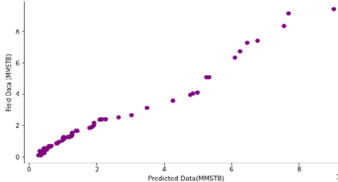
The random state parameter is used to initialize the random number generator used in the train_test_split process. Simply put, the same random splitting will occur each time the algorithm is run with the same random state value. To visualize the result obtained from the model developed, the matplotlib module was imported. The relationship between the predicted variable and the field data in normalized form is shown in Figure 6. The error plot for the newly developed SVR model is presented in Figure 7.
From the obtained results, the expression for predicting oil in place for oil rim reservoirs is provided in Equation 15.
( ) * * ( , ) SVR i i OIP y K x x b α =∑ + (15)
where i α are the dual coefficients (Lagrange multiplier) associated with each support vector ix ; b is the bias of the model; y is the target value for each support vector ix ; ( ) , i K x x is the kernel function that computes the similarity or inner product between the support vector ix and the input ; x and b is the bias term, which are all determined during the training phase of the SVR model. The corresponding values for the developed SVR model is presented in Tables 5 and Table 6.
| x 1 | x 2 | x 3 | x 4 | x 5 | x 6 | b |
|---|---|---|---|---|---|---|
| 0 | 0 | 0 | 0 | 0 | 0 | 0.0996 |
| 0.7878 | 0.1336 | 0.75 | 0.4412 | 0.0104 | 0.3038 | |
| 1 | 0.2434 | 0.95 | 0.7794 | 0.0454 | 0.782 | |
| 0.7878 | 0.1333 | 0.75 | 0.4412 | 0.0103 | 0.3036 | |
| 0.8585 | 0.1473 | 0.8 | 0.4559 | 0.0123 | 0.3789 |
Table 5: Support vectors and bias of the developed SVR model.
| α 1 | α 2 | α 3 | α 4 | α 5 |
|---|---|---|---|---|
| 0.1291 | -0.0207 | 0.9756 | -1 | -0.084 |
Table 6: Dual Coefficients of the developed SVR model.
The choice of kernel function determines how the SVR model captures the non-linear relationships in the data. This kernel function transforms the input data into a higher- dimensional feature space. The correlation for the linear kernel function is expressed in Equation 16.
$$ K \left(x _ {i}, x\right) = x _ {i} ^ {*} x \tag {16} $$
where K denotes the kernel function; ix is the support vector and x represents the input data.
Development of the Multiple Linear Regression Model
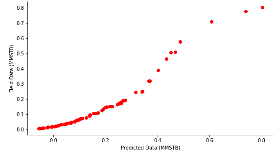
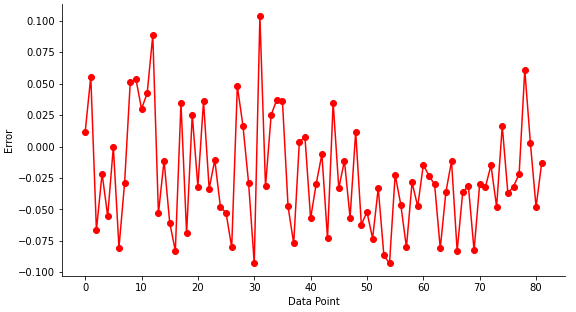
Similar in process to the SVR model, The MLR model was developed following the same procedure. However, the MLR object was imported from sklearn.linear_model library. The dataset was split into the x and y variables, with x being the six input parameters and y the output parameter (oil in place). The x and y dataset were scaled using the StandardScaler object imported from sklearn.preprocessing library. Data scaling is necessary to prevent numerical instability, because if the data points varies far from each other, the performance of the model will be poor. Afterwards, the dataset was partitioned into test size of 35% and training data of 65% to get the best performance result, the random state was also specified to the forty-two. Figure 8 shows the relationship between the predicted data and the field data for oil in place for the MLR model. The error distributions for the newly developed MLR model are shown in the error plot presented in Figure 9.
From the developed MLR model, the equation for estimating oil in place for oil rim reservoirs is given in Equation 17.
$$ O I P _ {M L R} = b _ {o} + b _ {1} h _ {o} + b _ {2} B _ {o} + b _ {3} \varphi + b _ {4} S _ {w} + b _ {5} A + b _ {6} m \tag {17} $$ where b0 represents intercept or the coefficient associated with a constant term; 1_b_ through 6_b_ denote the coefficients associated with the input variables ( , , , , , o o w h B S A m ϕ ). Thus, the coefficients of the developed model are presented in Table 7.
| b o | b 1 | b 2 | b 3 | b 4 | b 5 | b 6 |
|---|---|---|---|---|---|---|
| 22067536.23 | -10602626.53 | 3404446.69 | 4062776.53 | 4086350.41 | -2245930.63 | 26417750.79 |
Table 7: Coefficients of the developed MLR model.
Sensitivity Analysis of the Developed ANN Model
Sensitivity analysis examines how changes in input variables or assumptions affect the output of a model or analysis. It helps to understand the robustness of results and identifies which factors have the most significant impact on the outcome. There are different methods used for sensitivity analysis namely: partial derivatives, connection weights algorithm, forward and backward stepwise addition input perturbation amongst others [39]. Olden, et al. [40] conducted a comparison and reported that the method of connection weights was the least biased among others. As a result, this study deployed the connection weights algorithm. The connection weights technique described by Olden, et al. [41] computes the sum of products of final weights of connections from input neurons to hidden neurons with connections from hidden neurons to output neurons for all input neurons. The relative importance of a given input variable is expressed in Equation 18.
$$ R I _ {i} = \sum_ {j = 1} ^ {n} I W _ {i} ^ {j} \times L W _ {1} ^ {2} \tag {18} $$ $$ \sum_ {j = 1} ^ {n} I W _ {i} ^ {j} \times L W _ {1} ^ {2} $$
denotes the total product of the
connection weights (output neuron to the hidden neuron), where 2 1 1 i RI represents the relative importance of a given input variable, j is the number of hidden neurons, and 2 1 LW is the weights of the output neuron. Hence, the result determined by the product sum, rank and weighting of the input parameters are summarized in presented in Table 8 through Table 10 and Figure 10.
| Oil Column Thickness | Oil Formation Volume Factor | Porosity | Water Saturation | Area | M-factor | Output | |
|---|---|---|---|---|---|---|---|
| Hidden Layer 1 | 0.685801 | 0.755557 | -0.16782 | 0.146391 | 1.598598 | 0.985223 | 1.97521 |
| Hidden Layer 2 | 0.606326 | -1.316169 | 0.221929 | -0.732829 | 0.587082 | -0.21037 | -7.40073 |
| Hidden Layer 3 | 0.607569 | 0.962716 | 0.035803 | 0.303653 | -3.88356 | -0.01166 | 6.771898 |
| Hidden Layer 4 | -1.022843 | -0.860526 | 0.921702 | 0.431266 | -0.14791 | 1.12337 | 0.399309 |
| Hidden Layer 5 | 0.779506 | 1.564678 | -0.78411 | -0.422652 | 0.809694 | -1.18806 | 0.391533 |
| Hidden Layer 6 | -0.559897 | 1.261749 | -0.19332 | 0.65746 | -5.71381 | 0.19068 | -9.44174 |
| Hidden Layer 7 | -0.772339 | -0.700345 | -0.29039 | 0.2471 | 0.138854 | 0.405154 | 1.811358 |
Table 8: Final connection weights.
| Oil column Thickness | Oil Formation Volume Factor | Porosity | Water Saturation | Area | M-factor | Output | |
|---|---|---|---|---|---|---|---|
| Hidden Layer 1 | 1.354601 | 1.492384 | 0.331477 | 0.289152 | 3.157567 | 1.946023 | 8.571205 |
| Hidden Layer 2 | 4.487254 | 9.740618 | 1.642434 | 5.423473 | 4.344835 | 1.5569 | 27.19551 |
| Hidden Layer 3 | 4.114396 | 6.519413 | 0.242453 | 2.056307 | 26.29908 | 0.078958 | 39.31061 |
| Hidden Layer 4 | 0.40843 | 0.343616 | 0.368044 | 0.172208 | 0.059063 | 0.448572 | 1.799933 |
| Hidden Layer 5 | 0.305202 | 0.612623 | 0.307005 | 0.165482 | 0.317022 | 0.465166 | 2.172499 |
| Hidden Layer 6 | 5.286403 | 11.9131 | 1.825286 | 6.207564 | 53.94833 | 1.800348 | 80.98104 |
| Hidden Layer 7 | 1.398983 | 1.268575 | 0.526 | 0.447587 | 0.251514 | 0.73388 | 4.626538 |
| Oil Column Thickness | Oil Formation Volume Factor | Porosity | Water Saturation | Area | M-factor | ||
| Hidden Layer 1 | 0.158041 | 0.174116 | 0.038673 | 0.033735 | 0.368392 | 0.227042 | |
| Hidden Layer 2 | 0.165 | 0.35817 | 0.060394 | 0.199425 | 0.159763 | 0.057248 | |
| Hidden Layer 3 | 0.104664 | 0.165844 | 0.006168 | 0.052309 | 0.669007 | 0.002009 | |
| Hidden Layer 4 | 0.226914 | 0.190905 | 0.204476 | 0.095675 | 0.032814 | 0.249216 | |
| Hidden Layer 5 | 0.140484 | 0.28199 | 0.141314 | 0.076171 | 0.145925 | 0.214115 | |
| Hidden Layer 6 | 0.06528 | 0.14711 | 0.02254 | 0.076655 | 0.666185 | 0.022232 | |
| Hidden Layer 7 | 0.302382 | 0.274195 | 0.113692 | 0.096743 | 0.054363 | 0.158624 | |
| Sum | 1.162765 | 1.592329 | 0.587257 | 0.630714 | 2.096449 | 0.930486 | |
| Rank | 3 | 2 | 6 | 5 | 1 | 4 |
Table 9: Connection weight products.
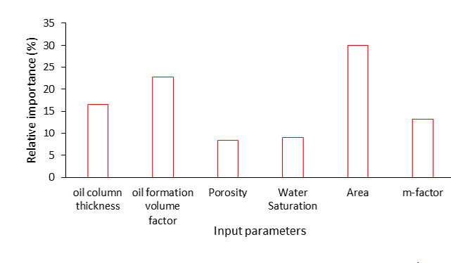
The result of sensitivity analysis presented in Figure 10 indicates that area extent of the oil rim reservoir had the greatest impact on the oil in place estimation with 29.94% followed by the oil formation volume factor (22.74%), oil column thickness (16.61%), m-factor (13.29%), water saturation (9.01%) and porosity (8.38%). It is worth noting that the sensitivity of the parameter reflects how the system’s performance varies when the parameter changes. The relative importance obtained in this study is as a result of the dataset gathered.
Model Comparison
Comparison Among Developed Models
To further ascertain the performance of the developed models, five (5) statistical analysis metrics namely – R-squared (R2), mean square error (MSE), root mean square error (RMSE), average absolute relative error (AARE) and average percent relative error (APRE) were used to assess the models. The comparison of the performance of the developed models is presented in Table 11.
| Models | R2 | MSE | RMSE | AAPRE | APRE | |
|---|---|---|---|---|---|---|
| This study (2023) | ANN | 0.9994 | 0.0001 | 0.0100 | 0.0081 | -0.0081 |
| SVR | 0.9157 | 0.0024 | 0.0489 | 97.6332 | -97.6332 | |
| MLR | 0.9793 | 0.0013 | 0.0360 | 17.7730 | -17.7730 |
Table 10: Comparison of developed models using statistical error tools.
It is well known that the higher the R2 values and the lower the MSE values, the better the model. From this inference, it can be concluded that the ANN model has the best performance. Figure 11 presents the developed models performance relative to the actual field data (in normalized form) plotted against each other, for some reservoirs.
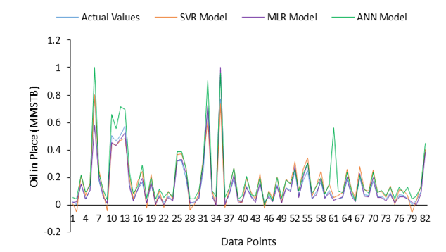
As may be seen in Figure 11, the developed ML models performed very well and may be used in the industry to estimate OIP for oil rim reservoirs in Niger Delta. Though there were cases of overestimation in some reservoirs caused by the ANN model but the errors were less than 20%. Also, the other two models (SVR and MLR) did perform well.
Comparison of the Newly Developed Models With Published Surrogate Models
Review of related literatures show that, apart from the conventional methods, there are little direct models for oil in place estimation. However, there are plethora of recovery factor correlations. These can therefore be related to the estimation of oil in place using Equation 19.
$$ R F = \frac {N _ {p}}{N} \tag {19} $$
where RF = Recovery factor (%), p N = cumulative net production (MMSTB) and = OIP (MMSTB).
However, based on an engineering standpoint, various assumptions, reverse calculations (at some point) were made to account for some parameters that were needed for the published surrogate models considered in this work, but not available in the dataset gathered. These parameters were then fitted into existing surrogate models to determine the OIP. Figures 12 and 13 show the comparison between the published related models, newly developed models and the field OIP data.
![Figure 12: Comparison between the newly developed models and Olamigoke-Isehunwa [42] model.](/fulltextimages/10863/fig_12.png)
The recovery factor correlation for vertical wells developed by Olamigoke and Isehunwa [42] was used to determine the recovery factor of the oil rim reservoirs in the Niger Delta of the gathered dataset. Thereafter, Equation 12 was employed to estimate the OIP in relation to the cumulative production data provided from the dataset used in this study. Figure 12 was plotted, considering 20 different reservoirs, and it can be noted that the developed ML models have excellent prediction as their data points were very close to the field (actual) data. Figure 12 also indicated that there was a point of underestimation for reservoir 12 using the Olamigoke and Isehunwa [42] model.
Another comparison was made using the OIP models developed by Tom, et al. [21]. The design of experiment (DOE)-based model was correlated with parameters in the gathered dataset to determine OIP values. These values were afterwards used to compare with the newly developed models and the field (actual) data. Figure 13 shows the comparison between the models.
![Figure 13: Comparison between the newly developed models and Tom, et al. [21] model.](/fulltextimages/10863/fig_13.png)
Evidently, reservoir 6 reveals that Tom, et al. [21] model made an overestimation of OIP for oil rim reservoirs. Also, reservoirs 10 through 13 had some degree of overestimation. This could be as a result of the unavailability of true reservoir data, and the effect of data randomization carried out in their study. Nonetheless, in general it can be seen that the developed ML models performed better. In terms of performance metrics, Table 12 shows the statistical errors for the newly developed models and the models from Tom, et al. [21].
| Models | R² | MSE | RMSE | |
|---|---|---|---|---|
| Tom, et al. [21] | DOE | 0.9971 | 0.0003 | 0.0172 |
| Tom, et al. [21] | ANN | 0.9241 | 0.0079 | 0.0891 |
| This study (2023) | ANN | 0.9994 | 0.0001 | 0.0100 |
| This study (2023) | SVR | 0.9157 | 0.0024 | 0.0489 |
| This study (2023) | MLR | 0.9793 | 0.0013 | 0.0360 |
Table 11: Statistical analysis of developed models for predicting oil in place with existing correlations.
The accuracy and precision of the developed models were furthermore evaluated using graphical representation of the percentage errors calculated from each models. These errors show the discrepancies of the predicted models from the actual (field) OIP data and are shown in Figures 14.
The lower the error margins of a model, the more closely the model is to the actual (field) data. Following this, it can be observed from Figures 14 that the MLR model had the least errors when compared to others. Negative error percentage indicates that the predicted value is smaller than the actual (OIP) value which means underestimation of those reservoirs in question.
![Figure 14: Comparison of errors discrepancies between the newly developed models, Olamigoke, et al. [42] and Tom, et al. [21] model.](/fulltextimages/10863/fig_14.png)
Conclusion
Estimation of oil in place is a crucial criterion for stakeholders and bidders to determine the prospect ranking and evaluation of a well before exploitation. For oil rim reservoirs in the Niger Delta, there are many different studies predominately on development and optimization of production. However, very few literature has been published on the estimation of oil in place. Since conventional methods for oil in place estimation are known to have some features hindering their predictive capabilities and applications, machine learning models – ANN, SVR, and MLR have been developed for estimation of oil in place for oil rim reservoirs in the Niger Delta.
Based on pairplots analysis of the various rock and fluid properties in the gathered dataset in python seaborn library, the knowledge of the parameters in volumetric method and the importance of other parameters, six (6) input variables were considered, namely; porosity (%), oil column thickness (ft), areal extent (acres), oil formation volume factor (bbl/ stb), gas cap size (m-factor), water saturation (%) to predict the (output) oil in place (MMSTB). The predictions of the developed models compared very well to the actual (field) results. The ANN model performed better than the SVR and MLR models. ANN model had an overall MSE of 0.0001, RMSE of 0.0100, APRE of -0.0081, AAPRE of 0.0081 and R2 of 0.9994. Also the SVR model had an overall R2 of 0.9157, MSE of 0.0024, RMSE of 0.0489, AARE of 97.6332 and an APRE of -97.6332. Lastly, the MLR model had an overall R2 of 0.9793, MSE of 0.0013, RMSE of 0.0360, AARE of 17.7730 and an APRE of -17.7730. The newly developed models in this study could offer stakeholders, investors and bidders a quick estimation of an oil rim reservoir potential before going further with exploitation and production.
References
-
Nasar AO, Abusaleem J, Tabar EM (2018) Estimation of Original Oil in Place for Belhedan Oil Field by Using Volumetric Method, Material Balance Equation Method, and Reservoir Simulation Method. Proceeding to Conference for Engineering, Science And Technology 1(2): 298-309.
-
Amadeo K, Brock TJ, Binder J (2022) What are Oil Reserves.
-
Short KC, Stauble AJ (1967) Outline of Geology of Niger Delta 1. American Association of Petroleum Geologists Bulletin 51(5): 761-779.
-
Corredor F, Shaw JH, Bilotti F (2005) Structural Styles in the Deep Water Fold and Thrust Belts of the Niger Delta. American Association of Petroleum Geologists Bulletin 89(6): 753-780.
-
Onukwuri AN, Azubuike II (2020) Improved Oil Recovery for Developed Oil Rim Reservoir Using Gas Blow Down Strategy A Case Study of Cefa Feild in Niger Delta. Int Res J of Adv Eng and Sci 5(2): 132-139.
-
Demirmen F (2007) Reserves Estimation The Challenge for the Industry. J of Pet Tech 59(5): 80-89.
-
Gehman MH, White DA (1979) Methods of Estimating Oil and Gas Resources. The American Association of Petroleum Geologists Bulletin 63(12): 2183-2192.
-
Anil KJ, Mao J, Mohiuddin KM (1996) Artificial Neural Network A Tutorial, Institute of Electrical and Electronics Engineers Access 29: 31-44.
-
Al BT, Mohammed B (2023) Mathematical Modification to the Classical Volumetric Method for Estimating Oil Reserves. Pet Petrochemical Eng J 7(1): 1-9.
-
Nwosu IE (2018) Volumetric and Material Balance Methods of Reserve Estimation A Comparative Study using Niger Delta Reservoirs. Int J of Eng Res and Adv Tech 4(9): 42-52.
-
Hossain MS, Hossain MAI, Akhter S (2011) A Study of Commonly used Conventional Methods for Gas Reserve Estimation. J of Chemical Eng 26 (1): 54-61.
-
Omoniyi OA, Adeolu S (2014) Material Balance and Decline Curve Analysis used as a Means for Estimating Reserves A Case Study of E1 and W1 Fields. Int J of Eng Res and Tech 7(3): 207-218.
-
Ahmed T, McKinney MP (2005) Advanced Reservoir Engineering. Gulf Professional Publishing, Burlington, United States of America, pp: 300.
-
Oloro J, Odu GO, Oyubu O (2011) Application of Decline Curve Analysis in Predicting the Life Span of a Well in Niger Delta Reservoir. Cont J of Earth Sciences 6(2): 1-8.
-
Downey L (2022) Decline Curve.
-
Dongmo ED, Zanga AA, Ngatcha DT, Metsebo J (2020) Comparison Study Between Different Methods Used in the Estimation of Reserves in Well F-12 of Volve Field. J of Ecology and Natural Resources 6(4): 78-94.
-
Horsfall OI, Uko ED, Ochoma U (2020) Deterministic Hydrocarbon Volume Estimation in the Onshore Fuba Field Niger Delta Nigeria. J of Applied Geology and Geophysics 8(1): 33-40.
-
Adeigbe OC, Odedere IF, Amodu OI (2018) Quantifying the uncertainty in the ultimate recoverable oil reserves using the Monte Carlo simulation techniques from ‘OWA’ Marginal Field, Onshore Niger Delta Nigeria. Geology Geophysics and Environment 44(4): 401-412.
-
Nnyeruka EC, Abbey VO (2016) Oil and Gas Reserve Estimation using Visual Basic 11.0. Academic Research International 7(5): 10-18.
-
Khisamov RS, Sarafov AF, Kalimullin AM, Dryagalkina AA (2018) Probabilistic Statistical Estimation of Reserves and Resources according to the International Classification SPE PRMS. Scientific and Tech J Georesources 20(3): 158-164.
-
Tom IU, Okon AN, Okologume WC (2020) Volumetric Approach Based DOE and ANN Models for Estimating Reservoirs Oil in Place. Int J of Sci and Eng Res 11(7): 873-883.
-
Anifowose FA, Abdulraheem A (2010) Prediction of Porosity and Permeability of Oil and Gas Reservoirs using Hybrid Computational Intelligence Models Paper. North Africa Technical Conference and Exhibition, pp: 14-17.
-
Mohaghegh SD (2011) Reservoir Simulation and Modeling Based on Artificial Intelligence and Data Mining AI&DM. J of Nat Gas Science and Eng 3(6): 697- 705.
-
Nyein CY, Hamada MMA (2019) Artificial Neural Network ANN Prediction of Porosity and Water Saturation of Shaly Sandstone Reservoirs. International Journal of the Physical Sciences 7(34): 5308-5313.
-
Vardian M, Nasriani HR, Faghihi R, Vardian A, Jowkar S (2016) Porosity and Permeability Prediction from Well Logs Using an Adaptive Neuro Fuzzy Inference System in a Naturally Fractured Gas-Condensate Reservoir. Energy Sources Part A Recovery Utilization and Environmental Effects 38(3): 435-441.
-
Ghareb HM, Ahmed E, Nyein CY (2018) Artificial Neural Network ANN Prediction of Porosity and Water Saturation of Shaly Sandstone Reservoirs. Adv in Applied Sci Res 9(2): 26-31.
-
Olayiwola T (2017) Application of Artificial Neural Network to Estimate Permeability from Nuclear Magnetic Resonance Log. Society of Petroleum Engineers Annual Technical Conference and Exhibition, pp: 9-11.
-
Agwu OE, Akpabio JU, Dosunmu A (2020) Artificial Neural Network Model for Predicting the Density of Oil Based Muds in High Temperature High Pressure Wells. J of Pet Exp and Prod Tech 10: 1081-1095.
-
Miri R, Sampaio J, Ashfar M, Lourenco A (2007) Development of Artificial Neural Networks to Predict Differential Pipe Sticking in Iranian offshore oil Fields. International Oil Conference and Exhibition Veracruz Mexico, pp: 27-30.
-
Sircar A, Yadav K, Rayavarapu K, Bist N, Oza H (2021) Application of Machine Learning and Artificial Intelligence in Oil and Gas Industry. Pet Res 6(4): 379- 391.
-
Bagheripour P, Gholami A, Asoodeh M (2014) Support Vector Regression between PVT Data and Bubble Point Pressure. J of Pet Exp and Prod Tech 1(5): 227-231.
-
Talebkeikhah M, Sadeghtabaghi Z, Shabani MA (2021) Comparison of Machine Learning Approaches for Prediction of Permeability using Well Log Data in the Hydrocarbon Reservoirs. J of Human Earth and Future 2(2): 82-99.
-
Mustafar IB, Razali RA (2011) Study on Prediction of Output in Oilfield Using Multiple Linear Regression. Int J of Applied Sci and Tech 1(4): 107-113.
-
Bayoka LR, Garris NA, Karimova GI (2019) Multiple Regression Model for Determining and Predicting the Viscosity of Crude Oils Mixture. Inst of Physics Publishing Conference Series Earth and Environmental Science 2(7): 1-7.
-
Elkatatny S, Mahmoud M (2018) Development of new correlations for the oil formation volume factor in oil reservoirs using Artificial Intelligent White Box Technique. Petroleum 4(2): 178-186.
-
Obah B, Livinus A, Ezugwu C (2012) Simplified Models for Forecasting Oil Production Niger Delta Oil Rim Reservoirs Case. Petroleum Technology Development Journal 2(2): 1-12.
-
Ukpong SE, Livinus A (2023) Application of a Simulation Approach to Develop Erosional Velocity Correlation for Wells in Oil Rim Reservoirs in the Niger Delta. SPE Nigeria Annual International Conference and Exhibition, Lagos, Nigeria.
-
Omeke J, Livinus A, Uche IN, Obah B, Ekeoma E (2010) A Proposed Cone Breakthrough Time for Horizontal Wells in Thin Oil Rim Reservoirs. Paper SPE 140743 presented at the 43rd SPE Conference.
-
Effiong AJ, Etim JO, Okon AN (2021) Artificial Intelligence Model for Predicting Formation Damage in Oil and Gas Wells. SPE Nigerian International Conference and Exhibition, Lagos, Nigeria.
-
Olden J, Joy M, Death R (2004) An Accurate Comparison of Methods for Quantifying Vraiable Importance in Artificial Neural Networks Using Simulated Data. J of Eco Model 178(3-4): 389-397.
-
Olden JD, Jackson DA (2002) Illuminating the black box Understanding Variable Contributions in Artificial Neural Networks. J of Eco Model 154(1-2): 135-150.
-
Olamigoke O, Isehunwa SO (2019) Primary Recovery Factor Correlations for Thin Oil Rims with Large Gas Caps. J of Eng Sci and Tech 14(4): 2359-2371.
- Nigeria’s Vulnerability in the Face of Global Energy Policy
- A Simulation Study of Investigation of Optimum Oil Production Performance by Applying Various Gas Injection Methods in Oil Reservoir
- Characterization of Permo-Triassic Reservoirs through Thermal Maturity Assessment of Westphalian Source Rocks in the Cheshire Basin
- Influence of Microwax on the Rheological and Thermal Behaviour of a Wax Crude Oil
- Real-Time Monitoring and Performance Optimization of Steam Injection in Heavy Oil Reservoirs Using Fiber Optic Sensing and Integrated Predictive Simulation Models
- Rapid On-Site Determination of the Total Petroleum Hydrocarbon Content of Soils by Handheld Fourier Transform Near-Infrared Spectroscopy: Development of a Global, Site- and Scanner- Independent Calibration Model