Pressurization Characteristics and Proppants Transport of Pulse Jet Fracturing with CFD-DEM Coupling Method
Hydraulic jet fracturing, which integrates hydraulic sand jet perforation and hydraulic fracturing, is widely used in the stimulation of low permeability reservoir. However, due to the complexity of the fluid-solid interaction, the effect of pressurization characteristics and proppants transport in the perforation hole are still unclear. Therefore, in this paper, the pressurization characteristics and proppants transport of pulse jet fracturing are investigated under different pressure amplitude, angular velocity, average pressure, nozzle diameter and perforation diameter with the CFD-DEM (Computational Fluid Dynamics and Discrete Element Method) coupled method. Results indicates that the effect of pressure amplitude, average pressure are positively related to the maximum velocity and maximum total pressure, while the effect of nozzle diameter is positively correlated with the maximum velocity, and the maximum total pressure has a relatively small effect. The effect of perforation diameter is negatively related to maximum velocity. It can be seen that pulsed jet fracturing can effectively relieve the large number of proppants blocking present around the perforated inlet of a single section of the pulse jet fracturing model (SPJFM). But when the proppants are of a certain size and the nozzle diameter is very small, it is difficult for the proppants to enter the perforation. And the smaller the diameter of the perforation, the less proppant enters the perforation, and some of the proppant appears in the annular section. By reasonably designing the optimal parameters, the pulsed jet can maximize the pressurization, helping optimize jet fracturing application parameters.
Introduction
China’s unconventional oil and gas resources are distinguished by huge reserves, widespread distribution, and deep burial, the active development of unconventional oil and gas resources is critical to ensuring the security of China’s energy supply [1]. Hydraulic fracturing has emerged as a significant technology for increasing output when producing unconventional oil and gas resources such as shale gas. It has the potential to form intricate fracture networks in unconventional reservoirs as well as boost the permeability of thick reservoirs. As one of the essential fracturing means for unconventional oil and gas, hydraulic jet fracturing technology has attracted more and more attention of scholars at home and abroad. Hydraulic jet fracturing completion technology has many advantages such as simple operation, safety and flexibility [2, 3, 4]. It has been widely used and studied in unconventional oil and gas exploitation. Recent studies show that hydraulic jet fracturing has an obvious effect on perforation pressurization, hydraulic sealing effect of annular section and improvement of sandblasting efficiency. The high-pressure jet during hydraulic fracturing enlarges the cracks in the rock, making the blasted holes larger and deeper, increasing the perforation pressure. At the same time, hydraulic fracturing is an effective way to stimulate the reservoir and ensure the economical production of natural gas.
Qu Hai, et al. [5] studied the effect of nozzle pressure drop, nozzle diameter, casing hole diameter and other factors on pore pressurization through indoor experiments. At the same time, jet fracturing technology has certain applications in the field of hydraulic sealing [6]. Qu Hai, et al. [7] used computational fluid dynamics methods to study the hydraulic seal pressure field in the process of hydraulic jet fracturing, and respectively revealed the effect law of hydraulic seal pressure field under the action of different factors, which provided scientific basis for the on-site construction of hydraulic jet fracturing process. Through experiments, Zhang [8] showed that the hydraulic sandblasting perforation velocity must meet the critical jet velocity, that is, the velocity when the rock is broken. The critical jet velocity at this time can achieve the best sand blasting perforation efficiency. In the process of hydro jet fracturing, the high-pressure jet will make the pressure in the pore channel higher than the annular section, thus acting as a jet pressurization in the pore channel. Fan, et al. [9] showed experimentally that the magnitude of annular pressure reduction was linearly increasing with the jet velocity and exponentially decreasing with the surrounding pressure. Through indoor tests, Xia, et al. [10] showed that the nozzle pressure drop and inlet ratio have a linear relationship with jet pressurization. Sheng, et al. [11] demonstrated through numerical simulation that the ratio of the pressure increase value of the jet in the hole to the inlet area presents a negative exponential decay law. Chen, et al. [12] showed through single-factor and multivariate sensitivity analysis that hydraulic fracturing can promote the development of low permeability hydrate reservoirs by combining reduced pressure with hot water injection. Ge, et al. [13] experimentally verified that high-pressure water jets break rocks more severely under high temperature conditions.
The high-pressure jet can form pulses in a variety of ways, and finally convert the high-pressure jet into a pulsed jet, improving the efficiency and accuracy of jet processing. Xue, et al. [14] studied the propagation of stress waves in rocks to reveal the rock breaking mechanism under pulsed water jets. The results show that with the gradual increase of the jet velocity, the influence area, propagation speed and attenuation rate of the stress wave increase. The pulsed injection cycle fracturing technology proposed by Cai, et al. [15] had the effect of cyclic pressurization and fracturing. They had achieved a good outcome of fracture network reconstruction in the high-pressure CO2 pulse cycle injection fracturing experiment. Cheng, et al. [16] studied the propagation law of pulsating water pressure in the pulsed hydraulic fracturing of coalbed methane reservoirs under different pulse frequencies and plugging rates through laboratory experiments. Zhang, et al. [17] showed that the acoustic emission (AE) signals in the low-pressure pulsating fracturing stage were relatively dispersed, and the pulsating energy promoted the development of micro-fractures through the new high-efficiency anti-reflection method of the coal seam in radial well-pulsating hydraulic fracturing. The AE signals are relatively concentrated in the high-pressure pulsating fracturing stage, and the pulse energy promotes the rapid extension of the main fracture. Liu, et al. [18] established a fracture conductivity model under a rod-shaped proppant to explore the fracture conductivity during pulse fracturing, providing a theoretical basis for combining rod-shaped proppant and pulse fracturing to improve productivity. Lu, et al. [19] studied the stress propagation and distribution law in fractured strata during pulsating hydraulic fracturing. Then they analyzed the influence mechanism of fracture fillings on the stress disturbance effect of pulsating hydraulic fracturing under different fracture spacing and focal frequency. At the same time, the distribution law of the minimum principal stress peak of coal seam under different loading modes, frequencies, amplitudes and confining pressures was explored to provide particular guidance for optimizing process parameters of pulsating hydraulic fracturing [20]. Liao, et al. [21] established a numerical model to study the propagation of hydraulic fractures under the condition that the horizontal wellbore is not collinear with the minimum horizontal principal stress. They applied the extended finite element method to the fluid-structure coupling of horizontal multi-stage fracturing, which is of great significance for optimizing the fracturing process. Dehkhoda, et al. [22]
showed that the pulsation frequency has a great influence on the damage degree of the rock target, and at the same time, the fracture propagation caused by impact causes rock failure depending on the pulse length. Liu, et al. [23] studied the effect of stress wave propagation on rock fragmentation when granite is investigated by pulsed water jets, and found that the two modes of rock fragmentation are caused by the combined effect of impact stress wave and the pulsating water wedge pressure. Wang, et al. [24] conducted a series of experiments to investigate the penetration characteristics of a low-frequency pulsed water jet impact and compared the failure modes of sandstone and granite rock samples. Their study greatly advanced the development of low-frequency liquid jet technology. Zhang, et al. [25] verified by experiments that the overall erosion ability of pulsed water jet is better than that of continuous water jet, which provides a reference for further optimization of pulsed water jet technology to break different rocks in the future.
Proppants play an essential role in the production process. Hari, et al. [26] conducted different experimental studies on sandstone formations to analyze the effect of various factors exacerbating the proppant breaking and embedding process. Proppant comes in a variety of shapes, and pulse fracturing in conjunction with rod-shaped proppant has been shown to reduce proppant flowback issues and boost well productivity. Proppants play a key role in hydraulic fracturing by enhancing fracture conductivity, which is often investigated via experimental or numerical model. Zhao, et al. [27] proposed a coupled CFD-DEM (Computational Fluid Dynamics-Discrete Element Method model) method to simulate the interaction between fluid and particles in granular media. The interaction between fluid and particle is considered by exchanging interaction forces. Studies have shown that the rolling resistance among particles has a greater relative pressure dip for a single-size case and a smaller relative pressure dip for a polydisperse case. Li, et al. [28] used DEM-CFD better to understand the dynamic characteristics of high-speed abrasive air jets. It is found that lower shape factors, and increased aerodynamic drag resulted in higher particle velocities, allowing abrasive particles to remain more centrally along the centerline of the jet axis, further affecting jet expansion. It has been discovered, however, that the form factor of the abrasive particles has no detectable effect on high-speed air flow. Zhu, et al. [29] built up proppant discrete element model and CFD (Computational Fluid Dynamics) numerical model to conduct study. It reveals the change mechanism of the diverting capacity of supporting cracks. Proppant placement in fracturing fractures can also seriously affect the post-fracturing production increase effect. Guo, et al. [30] consider accurately capture particle movement of CFD/DEM coupling method, building a complex fracture three-dimensional model, to explore the effect of proppant transport and placement under the impact of different parameters. The results of Cai, et al. [31] show that increasing the nozzle pressure drop and increasing the nozzle diameter are beneficial to enhance the impact effect of the jet on rocks, and increasing the nozzle diameter can also increase the impact range of the jet. Increasing the spray distance will cause the high-pressure CO$_2$ jet to greatly reduce the impact force on the rock surface. The research results are conducive to the further improvement of the drilling technology of underbalanced high-pressure gas. Pulse injection fracturing technology displays an excellent enhancement.
However, due to the complexity of the fluid-solid interaction, the effect of pressurization characteristics and proppants transport in the perforation hole are still unclear. Therefore, to address the above concerns, a CFD/DEM coupling model of pulse jet fracturing in the horizontal wellbore is established to explore the flow field and proppants transport position of pulse jet. The variation of pressurization characteristics and proppants transport under different factors, such as pulse jet pressure amplitude, angular velocity, average pressure, nozzle diameter and perforation diameter, is studied. The research can help optimize jet fracturing application parameters.
**Methodology and Validation of CFD/DEM Coupling Model**
**CFD/DEM Coupling Method**
In the process of pulsed jet fracturing, the interaction between fracturing fluid and proppants in wellbore and perforation is a complex fluid-solid coupling problem. As a typical two-phase flow of pulsed jet fracturing, both solid domain and fluid domain solutions should be established. The main governing equations are as follows:
The Governing Equations of the Fluid Domain: The continuity equation in differential form is established with the micro-element control body. The mass of the net outflow of the micro-element body must be equal to the mass reduction in the micro-element body, according to the law of mass conservation. Equation (1) can be obtained as follows:
Continuity equation:
$$\frac{\partial \rho}{\partial t} + \nabla \cdot (\rho \vec{u}) = 0$$
Equation (1) is the partial differential equation form of the continuity equation based on the infinitesimal micro cluster model with fixed spatial position. The law of conservation of momentum is a law that any flowing system must satisfy. Fluid micro cluster are subjected to volumetric and surface forces in the x, y, and z directions. The total force is obtained by adding the volume and surface forces in the three directions. According to the conservation of mass, we can get equation (2) as follows:
Momentum equation:
$$-\frac{\partial \rho}{\partial x} + \frac{\partial \tau_{xx}}{\partial x} + \frac{\partial \tau_{yx}}{\partial y} + \frac{\partial \tau_{zx}}{\partial z} + \rho f_x = \frac{\partial (\rho u)}{\partial t} + \nabla \cdot (\rho u V)$$
where $t$ is the time, $s$; $\rho$ is the particle density, kg/m$^3$, $u$ is the fluid velocity vector, m/s, $\tau$ is the viscous stress tensor.
The law of conservation of energy is the fundamental law that must be satisfied by the heat exchange system. It can be expressed as: The power of volume force, surface force, and net heat flow into the micro-element body are added to determine the rate of energy change in the micro-element body. Equation (3) can be obtained as follows:
$$\rho \frac{De}{Dt} = \rho q + \frac{\partial}{\partial x} \left( \lambda \frac{\partial T}{\partial x} \right) + \frac{\partial}{\partial y} \left( \lambda \frac{\partial T}{\partial y} \right) + \frac{\partial}{\partial z} \left( \lambda \frac{\partial T}{\partial z} \right) - \rho \left( \frac{\partial u}{\partial x} + \frac{\partial u}{\partial y} + \frac{\partial u}{\partial z} \right) + \tau_{xx} \frac{\partial u}{\partial x} + \tau_{yy} \frac{\partial u}{\partial y} + \tau_{zz} \frac{\partial u}{\partial z} + \tau_{xy} \frac{\partial u}{\partial x} + \tau_{zy} \frac{\partial u}{\partial y} + \tau_{xz} \frac{\partial u}{\partial z} + \tau_{yz} \frac{\partial u}{\partial y} + \tau_{zz} \frac{\partial u}{\partial y} + \tau_{zz} \frac{\partial u}{\partial y} + \tau_{zz} \frac{\partial u}{\partial y} + \tau_{zz} \frac{\partial u}{\partial y} + \tau_{zz} \frac{\partial u}{\partial y} + \tau_{zz} \frac{\partial u}{\partial y} + \tau_{zz} \frac{\partial u}{\partial y} + \tau_{zz} \frac{\partial u}{\partial y} + \tau_{zz} \frac{\partial u}{\partial y} + \tau_{zz} \frac{\partial u}{\partial y} + \tau_{zz} \frac{\partial u}{\partial y} + \tau_{zz} \frac{\partial u}{\partial y} + \tau_{zz} \frac{\partial u}{\partial y} + \tau_{zz} \frac{\partial u}{\partial y} + \tau_{zz} \frac{\partial u}{\partial y} + \tau_{zz} \frac{\partial u}{\partial y} + \tau_{zz} \frac{\partial u}{\partial y} + \tau_{zz} \frac{\partial u}{\partial y} + \tau_{zz} \frac{\partial u}{\partial y} + \tau_{zz} \frac{\partial u}{\partial y} + \tau_{zz} \frac{\partial u}{\partial y} + \tau_{zz} \frac{\partial u}{\partial y} + \tau_{zz} \frac{\partial u}{\partial y} + \tau_{zz} \frac{\partial u}{\partial y} + \tau_{zz} \frac{\partial u}{\partial y} + \tau_{zz} \frac{\partial u}{\partial y} + \tau_{zz} \frac{\partial u}{\partial y} + \tau_{zz} \frac{\partial u}{\partial y} + \tau_{zz} \frac{\partial u}{\partial y} + \tau_{zz} \frac{\partial u}{\partial y} + \tau_{zz} \frac{\partial u}{\partial y} + \tau_{zz} \frac{\partial u}{\partial y} + \tau_{zz} \frac{\partial u}{\partial y} + \tau_{zz} \frac{\partial u}{\partial y} + \tau_{zz} \frac{\partial u}{\partial y} + \tau_{zz} \frac{\partial u}{\partial y} + \tau_{zz} \frac{\partial u}{\partial y} + \tau_{zz} \frac{\partial u}{\partial y} + \tau_{zz} \frac{\partial u}{\partial y} + \tau_{zz} \frac{\partial u}{\partial y} + \tau_{zz} \frac{\partial u}{\partial y} + \tau_{zz} \frac{\partial u}{\partial y} + \tau_{zz} \frac{\partial u}{\partial y} + \tau_{zz} \frac{\partial u}{\partial y} + \tau_{zz} \frac{\partial u}{\partial y} + \tau_{zz} \frac{\partial u}{\partial y} + \tau_{zz} \frac{\partial u}{\partial y} + \tau_{zz} \frac{\partial u}{\partial y} + \tau_{zz} \frac{\partial u}{\partial y} + \tau_{zz} \frac{\partial u}{\partial y} + \tau_{zz} \frac{\partial u}{\partial y} + \tau_{zz} \frac{\partial u}{\partial y} + \tau_{zz} \frac{\partial u}{\partial y} + \tau_{zz} \frac{\partial u}{\partial y} + \tau_{zz} \frac{\partial u}{\partial y} + \tau_{zz} \frac{\partial u}{\partial y} + \tau_{zz} \frac{\partial u}{\partial y} + \tau_{zz} \frac{\partial u}{\partial y} + \tau_{zz} \frac{\partial u}{\partial y} + \tau_{zz} \frac{\partial u}{\partial y} + \tau_{zz} \frac{\partial u}{\partial y} + \tau_{zz} \frac{\partial u}{\partial y} + \tau_{zz} \frac{\partial u}{\partial y} + \tau_{zz} \frac{\partial u}{\partial y} + \tau_{zz} \frac{\partial u}{\partial y} + \tau_{zz} \frac{\partial u}{\partial y} + \tau_{zz} \frac{\partial u}{\partial y} + \tau_{zz} \frac{\partial u}{\partial y} + \tau_{zz} \frac{\partial u}{\partial y} + \tau_{zz} \frac{\partial u}{\partial y} + \tau_{zz} \frac{\partial u}{\partial y} + \tau_{zz} \frac{\partial u}{\partial y} + \tau_{zz} \frac{\partial u}{\partial y} + \tau_{zz} \frac{\partial u}{\partial y} + \tau_{zz} \frac{\partial u}{\partial y} + \tau_{zz} \frac{\partial u}{\partial y} + \tau_{zz} \frac{\partial u}{\partial y} + \tau_{zz} \frac{\partial u}{\partial y} + \tau_{zz} \frac{\partial u}{\partial y} + \tau_{zz} \frac{\partial u}{\partial y} + \tau_{zz} \frac{\partial u}{\partial y} + \tau_{zz} \frac{\partial u}{\partial y} + \tau_{zz} \frac{\partial u}{\partial y} + \tau_{zz} \frac{\partial u}{\partial y} + \tau_{zz} \frac{\partial u}{\partial y} + \tau_{zz} \frac{\partial u}{\partial y} + \tau_{zz} \frac{\partial u}{\partial y} + \tau_{zz} \frac{\partial u}{\partial y} + \tau_{zz} \frac{\partial u}{\partial y} + \tau_{zz} \frac{\partial u}{\partial y} + \tau_{zz} \frac{\partial u}{\partial y} + \tau_{zz} \frac{\partial u}{\partial y} + \tau_{zz} \frac{\partial u}{\partial y} + \tau_{zz} \frac{\partial u}{\partial y} + \tau_{zz} \frac{\partial u}{\partial y} + \tau_{zz} \frac{\partial u}{\partial y} + \tau_{zz} \frac{\partial u}{\partial y} + \tau_{zz} \frac{\partial u}{\partial y} + \tau_{zz} \frac{\partial u}{\partial y} + \tau_{zz} \frac{\partial u}{\partial y} + \tau_{zz} \frac{\partial u}{\partial y} + \tau_{zz} \frac{\partial u}{\partial y} + \tau_{zz} \frac{\partial u}{\partial y} + \tau_{zz} \frac{\partial u}{\partial y} + \tau_{zz} \frac{\partial u}{\partial y} + \tau_{zz} \frac{\partial u}{\partial y} + \tau_{zz} \frac{\partial u}{\partial y} + \tau_{zz} \frac{\partial u}{\partial y} + \tau_{zz} \frac{\partial u}{\partial y} + \tau_{zz} \frac{\partial u}{\partial y} + \tau_{zz} \frac{\partial u}{\partial y} + \tau_{zz} \frac{\partial u}{\partial y} + \tau_{zz} \frac{\partial u}{\partial y} + \tau_{zz} \frac{\partial u}{\partial y} + \tau_{zz} \frac{\partial u}{\partial y} + \tau_{zz} \frac{\partial u}{\partial y} + \tau_{zz} \frac{\partial u}{\partial y} + \tau_{zz} \frac{\partial u}{\partial y} + \tau_{zz} \frac{\partial u}{\partial y} + \tau_{zz} \frac{\partial u}{\partial y} + \tau_{zz} \frac{\partial u}{\partial y} + \tau_{zz} \frac{\partial u}{\partial y} + \tau_{zz} \frac{\partial u}{\partial y} + \tau_{zz} \frac{\partial u}{\partial y} + \tau_{zz} \frac{\partial u}{\partial y} + \tau_{zz} \frac{\partial u}{\partial y} + \tau_{zz} \frac{\partial u}{\partial y} + \tau_{zz} \frac{\partial u}{\partial y} + \tau_{zz} \frac{\partial u}{\partial y} + \tau_{zz} \frac{\partial u}{\partial y} + \tau_{zz} \frac{\partial u}{\partial y} + \tau_{zz} \frac{\partial u}{\partial y} + \tau_{zz} \frac{\partial u}{\partial y} + \tau_{zz} \frac{\partial u}{\partial y} + \tau_{zz} \frac{\partial u}{\partial y} + \tau_{zz} \frac{\partial u}{\partial y} + \tau_{zz} \frac{\partial u}{\partial y} + \tau_{zz} \frac{\partial u}{\partial y} + \tau_{zz} \frac{\partial u}{\partial y} + \tau_{zz} \frac{\partial u}{\partial y} + \tau_{zz} \frac{\partial u}{\partial y} + \tau_{zz} \frac{\partial u}{\partial y} + \tau_{zz} \frac{\partial u}{\partial y} + \tau
m
| C ρA d p | V s |
|---|
Schiller-Nauman correlation is applicable to spherical solid particles, liquid droplets and small diameter bubbles. The settings are:
( ) 24 0.687 3 1 0.15Re Re 10 p p Rep d 3 0.44 Re 10 p
$$ C _ {\mathrm {d}} = \left\{ \begin{array}{l l} \frac {2 4}{\mathrm {R e} _ {\mathrm {p}}} \left(1 + 0. 1 5 \mathrm {R e} _ {\mathrm {p}} ^ {0. 6 8 7}\right) & \mathrm {R e} _ {\mathrm {p}} \leq 1 \\ \end{array} \right. $$ (15) >
| ρ | V s | D p |
|---|
The pressure gradient force _F_p in equation (7) is defined as:
p p static F V P = − ∇ (17) where _V_p is the volume of particles, m3. And Ñ_P_static is the gradient of static pressure in the continuous phase.
The virtual mass force _F_vm in equation (7) is defined as:
$$ F _ {\mathrm {v m}} = C _ {\mathrm {v m}} \rho V _ {\mathrm {p}} \left(\frac {D v}{D t} - \frac {d v _ {\mathrm {p}}}{d t}\right) $$ (18) where _C_vm is the virtual mass coefficient. The default value of 0.5 for this coefficient is for a sphere with uniform, inviscid, incompressible flow.
The gravity _F_g in equation (8) is defined as:
$$ F _ {\mathrm {g}} = m _ {\mathrm {p}} g \tag {19} $$
where g is the gravitational acceleration vector, m/s2.
The force _F_MRF in the moving reference coordinate system in Formula (8) is defined as:
( ) ( ) 2 p p MRF F m r v ω ω ω = × × + × (20)
where ω is the angular velocity vector of the rotation reference coordinate system, rad/s. And r is the distance vector to the rotation axis, m.
The coulomb force _F_Co in equation (8) is defined as:
$$ F _ {\mathrm {C o}} = q E \tag {21} $$
The user-defined volume force Fu in equation (8) is defined
as:
$$ F _ {\mathrm {u}} = V _ {\mathrm {p}} f _ {\mathrm {u}} \tag {22} $$
where fu is the volume force per unit volume specified, N/m3.
CFD/DEM Coupling Model
Geometry of Numerical Model: The numerical model of pulse jet fracturing, which is composed of the pulse jet fracturing tool, wellbore annular and perforation, is first established by using CFD-DEM coupling method, as shown in Figure 1(a). To investigate the flow characteristic of the fracturing fluid and proppants, a single section of the numerical model is selected as the research goal Figure 1(b), which is named as a single section of the pulse jet fracturing model (SPJFM). The internal chamber of the single section of the pulse jet fracturing tool (SPJFT), the inlet channel section of the nozzle, the convergence section of the nozzle, the outlet channel section of the nozzle, the wellbore annulus section, and the perforation section are all included in the meshing results of the SPJFM, which are displayed in Figure 1(c). The internal chamber of the SPJFT is a cylindrical shape, with a diameter of 40mm and a length of 40mm (Figure 1(b) and Figure 1(c)). The cylindrical inlet channel section of nozzle has a 10mm diameter and a 16mm length, connecting with SPJFT. The conical convergence section of nozzle has a length of 7mm, with a convergence angle of 13.5°. The outlet section of nozzle has a 4mm diameter and a 2mm length. The high- pressure fracturing fluid would come out from the nozzle outlet into the wellbore annular, which has an inner diameter of 90 mm and an outer diameter of 114.3 mm. And then the jet will pressurize in the perforation section with a diameter of 15mm and length of 88.85mm. The distance between the perforation outlet and the referenced axis of the SPJFT is 146mm. The simulation boundary conditions at the inlet and outlet of SPJFM is both set as pressure boundary, and the numerical wall is all smooth wall. The prismatic layer grid and boundary layer grid are used to mesh the fluid model, and the ultimate number of grids is 146376 (Figure 1(c)).
Boundary Modeling of CFD-DEM: The Reynold Average Navier-Stokes (RANS) model and the k-turbulence model are used for modeling in this study, and the implicit unsteady solver is used for solution. The simulation model establishes the CFD-DEM coupling model to investigate the inter- phase interactions in the SPJFM channel. In the inter-phase interactions, consider the four typical interactions: particle and particle, particle and boundary, particle and fluid. In the parameters interaction between particle and particle, including the linear spring settings and rolling resistance, are decided based on many times practice. The ratio factor of rolling resistance is 0.001, and the linear spring’s tangential and normal stiffness are 50,000 N/m. The equivalent diameter of the proppants is 0.18 mm. The drag coefficient is calculated by using the Schiller-Nauman model, the virtual mass is set to 0.5 kg and the volume forces is set into 0 N/ mm3. The model parameters of the SPJFM is illustrated as shown in Table 1.
proppants size Young’s modulus (MPa)
- Dynamic viscosity
- (Pa•s)
- Annulus pressure
- Outlet pressure
- Nozzle diameter (mm)
- Perforation diameter (mm)
- Density (kg/m3)
- Inlet pressure (MPa)
- (MPa)
- (MPa)
- 1500
- 0.9
- (
- ) m
- 0
- 2
- P sin ft
- P π
- +
- +P0
- 15
- 10
- 4
- 15
- 1500
- 0.18
- 5.31×10⁴
- 0.294
Table 3: Fluid properties and other parameters.
$$ P _ {\mathrm {j}} = P _ {\mathrm {m}} \sin \left(2 \pi f t\right) + P _ {0} \tag {23} $$ Among them, the pressure amplitude _P_m is 15MPa, the angular velocity ω is 1rad/s, the average pressure _P_0 is 45MPa, and the outlet is set to the pressure outlet
| Number | Pressure amplitude (MPa) | Angular velocity (rad/s) | Average pressure (MPa) | Nozzle diameter (mm) | Perforation diameter (mm) |
|---|---|---|---|---|---|
| 0 | 15 | 1 | 45 | 4 | 15 |
| 01-Jan | 5 | 1 | 45 | 4 | 15 |
| 01-Feb | 10 | 1 | 45 | 4 | 15 |
| 01-Mar | 20 | 1 | 45 | 4 | 15 |
| 02-Jan | 15 | 0.1 | 45 | 4 | 15 |
| 02-Feb | 15 | 10 | 45 | 4 | 15 |
| 02-Mar | 15 | 0.01 | 45 | 4 | 15 |
Table 4: Specific simulation scheme (bold item is the basical group).
| 03-Jan | 15 | 1 | 35 | 4 | 15 |
|---|---|---|---|---|---|
| 03-Feb | 15 | 1 | 55 | 4 | 15 |
| 03-Mar | 15 | 1 | 65 | 4 | 15 |
| 04-Jan | 15 | 1 | 45 | 0.5 | 15 |
| 04-Feb | 15 | 1 | 45 | 1 | 15 |
| 04-Mar | 15 | 1 | 45 | 2 | 15 |
| 05-Jan | 15 | 1 | 45 | 4 | 10 |
| 05-Feb | 15 | 1 | 45 | 4 | 20 |
| 05-Mar | 15 | 1 | 45 | 4 | 25 |
| non-pulse | 15 | 0 | 45 | 4 | 15 |
Table 5: Specific simulation scheme (bold item is the basical group).
Mesh Independence and Validation
numbers determines the optimal number of meshes for all subsequent simulations and studies. The Table 3 shows the results comparison of velocity and total pressure relative error under different mesh numbers.
Mesh Independence: We should verify the mesh independence first. Comparing the results of different mesh
| Number of Grids (million) | Velocity (m/s) | Velocity error (%) | Total Pressure (MPa) | Total Pressure Error (%) |
|---|---|---|---|---|
| 14 | 186.99 | 0 | 32.03 | 0 |
| 8 | 168.86 | 9.7 | 27.61 | 13.82 |
| 10 | 177.9 | 4.86 | 29.76 | 7.1 |
| 12 | 178.67 | 4.5 | 30.01 | 6.3 |
| 16 | 189.02 | 1.1 | 32.51 | 1.5 |
| 18 | 196.21 | 4.7 | 34.25 | 6.5 |
| 20 | 198.92 | 5.99 | 35.05 | 8.59 |
Table 6: Comparison of simulation results with different number of meshes.
Validation: The pressure drop at the nozzle is changed by changing the pressure amplitude _P_m at the inlet and the average pressure _P_0 accordingly. Qu, et al. [32] studied the pressure distribution in the perforation under different nozzle pressure drop by setting the pressure of the nozzle in the annulus section to 15MPa. The study showed that the nozzle diameter is constant, and the pressure in the perforation increased with the nozzle pressure drop. In our study, the nozzle inlet pressure is 40MPa, the annular pressure is 15MPa, and the pressure drop of the nozzle is 25MPa. The overall pressure trend is similar to that obtained by Qu, et al. [32], Cheng, et al. [33] and Shi, et al. [34]. It is manifested as the pressure decreases first as the axial distance increases, and then gradually rises to the same as the outlet pressure after being reduced to the minimum pressure, confirming the model’s accuracy (Figure 3).
![Figure 3: Comparison results on pressure of our study with Qu, et al. [33] (The annular pressure is 15MPa and the pressure drop of nozzle is 25MPa), Cheng, et al. [34] (The nozzle inlet pressure is 55MPa, the annular pressure is 20MPa and the pressure drop of nozzle is 35MPa) and Shi, et al. [35] (The pressure drop of nozzle is 25MPa) under different conditions.](/fulltextimages/11356/fig_3.png)
Figure 3: Comparison results on pressure of our study with Qu, et al. [33] (The annular pressure is 15MPa and the pressure drop of nozzle is 25MPa), Cheng, et al. [34] (The nozzle inlet pressure is 55MPa, the annular pressure is 20MPa and the pressure drop of nozzle is 35MPa) and Shi, et al. [35] (The pressure drop of nozzle is 25MPa) under different conditions.
Results and Discussion
Effect of Pressure Amplitude (Pm)
The Variation of Jet Velocity (V): Figure 4 shows the velocity variation at wellbore section and perforation section velocity under different pressure amplitude. The results indicated that the maximum velocity along the jet axis sharply rises as the pressure amplitude increases. When the pulse pressure amplitude is 65MPa, the velocity of jet core reaches a maximum value of 269.9m/s. It is pointed out that the jet velocity is 135m/s obtained at the position of 21.44mm along the jet axis, which is equivalent value of 0.5_V_max at the position of 21.23% jet length. For all cases, the maximum velocity all rapidly reduced to the same value at the outlet of the perforation. The maximum velocity of the jet along the perforation inlet to the perforation outlet along the jet axis is gradually decreasing under the same pressure amplitude. And the maximum jet velocity increases with the pressure amplitude increases. Compared the pulse jet and non-pulse jet, it is found that when the pressure amplitude _P_m is 15MPa, the jet velocity of different perforated positions in SPJFT is greater than non-pulsed under this parameter.
In order to explore the velocity variation deeply, Figure 5 shows the variation of jet velocity along the X axis to various distance under different pressure amplitudes. It is found that when the pulse pressure amplitude increases from 50MPa to 65MPa, the maximum velocity amplitude varied from 234.7m/s to 269.9m/s, reaching increment of 15% in the maximum velocity amplitude. When the pressure amplitude _P_m has the maximum value of 15MPa, the maximum velocity of pulse case and non-pulse case is 258.72m/s and 221.70m/s respectively. For all cases, the maximum velocity rapidly reduced to 17m/s at the outlet section of the perforation. The maximum velocity reduction of the pulsed case is greater than the non-pulsed case under the same pressure amplitude.
The Variation of Total Pressure (P): The variation of total pressure at wellbore section and perforation section, respectively, under different pressure amplitude is shown in Figure 6. It can be seen that the maximum total pressure along jet axis steeply rises as the pressure amplitude increasing.
When the pulse pressure amplitude reaches to the maximum jet pressure amplitude of 65MPa, the total pressure of jet core reaches the maximum value of 61.7MPa. It is pointed out that the jet total pressure is 30.85MPa at the position of 15.23mm along the jet axis, which is correspondingly the
0.5_P_max at the 15.08% of the entire jet length. Particularly, at the outlet of the perforation, the maximum total pressure of all case rapidly reduced to the same value because of the same outlet pressure boundary setting. The maximum total pressure of the jet along the perforation axis has gradual reduction under the same pressure amplitude according to the color map in Figure 6(a). And when the pressure amplitude varied from 50MPa to 65MPa, it is found that there is a significant increasing of total pressure. Compared the pulse jet fracturing and non-pulse jet fracturing, the results reveal that the total pressure of pulse jet fracturing in SPJFM is greater than that of non-pulsed jet fracturing.
It is necessary to investigate the total pressure variation along the X axis under different pressure amplitudes (Figure 7). According to Figure 7, it is found that when the pulse pressure amplitude rises from 50MPa to 65MPa, the maximum total pressure has a 25.7% increment, rising from 49.1MPa to 61.7MPa. When the pressure amplitude _P_m has the value of 15MPa, we could obtain the maximum value of total pressure of 44.9MPa in non-pulse case. And the maximum value of total pressure of 57.5MPa in pulse case, which is 4.1% larger than the non-pulse case at the same jet parameters. Thereby, we can conclude that the total pressure reduction of pulsed case is always more significant than the non-pulse case under the same pressure amplitude.
Proppants Transport in the SPJFM: Figure 8 shows the proppants transport in the SPJFM under different pressure amplitudes. Compared the results under different amplitude pressure, it can be seen that there are 67, 64, 57 and 65 proppants accessing in the perforation, respectively. And the proportion of proppants entering the perforation is 22.3%, 21.3%, 19% and 21.7%, respectively. It is concluded that the number of transporting proppants would decrease firstly and then increase finally, with increasing amplitude pressure. As a compared group, it is interesting that the 52 proppants, which is 16.67% proportion of total proppants, transport into the perforation under the non-pulsed pressure of 45MPa. Also, it can be seen that there is a large number of proppants blocking the perforation inlet of the SPJFM. The number of blocking proppants at the perforation inlet of non-pulse jet fracturing is more obvious than that of pulsed case jet fracturing, which means the pulse jet could relieve the proppants blocking in the perforation entrance section.
Effect of Angular Velocity (Ω)
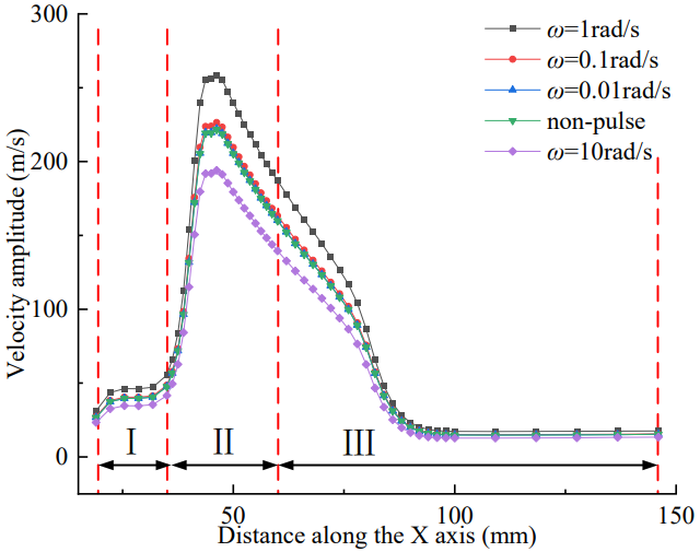
The Variation of Jet Velocity (V): Figure 9 shows the influence of angular velocity on jet velocity at wellbore and perforation section. The results suggest that the jet core velocity reaches a maximum value of 258.7 m/s when the angular velocity ω is 1 rad/s, and the jet velocity is 129.35m/s at 19.85mm along the jet axis, which is equivalent to 0.5_V_max at the position of 19.65% jet length. There is a smaller value of jet velocity than all others when the angular velocity ω is 10 rad/s. The jet velocity is 97.05 m/s at the position of 12.47mm along the jet axis, which is correspondingly the 0.5_V_max at the 12.35% of the entire jet length. As can be seen from Figure 9(b), when the angular velocity ω is 1rad/s, the velocity of jet core reached the maximum value at the nozzle outlet, and the velocity of the jet has the most clearly downward trend through the entire perforation. When the angular velocity ω is 10rad/s, there is a minimum value at the nozzle outlet. It is concluded that when the angular velocity varies from 0.01rad/s to 10rad/s, the maximum velocity increases firstly and then decrease. The comparison between pulse jet fracturing and non-pulse jet fracturing indicates that at a pulsed pressure amplitude of 60MPa, the jet velocity of different perforated positions in SPJFT is greater than that of the non-pulsed jet under the same angular velocity.
Figure 9: The influence of angular velocity on jet velocity at wellbore and perforation section. (Pm=15MPa; P0=45MPa; d=4mm; Dp=15mm) Figure 10 shows the variation of jet velocity along the X axis to various distances under different angular velocities so as to explore the angular velocity variation deeply. It is pointed out that the maximum velocity that can be achieved by the jet varies at different angular velocities. When the angular velocity ω is 1rad/s, 10rad/s, the maximum velocity of the jet is 258.7 m/s and 194.1 m/s, respectively. And the difference is 33.3%. Thus, we can conclude that there is an optimal angular velocity to get the maximum value of jet velocity.
The Variation of Total Pressure (P): Figure 11(a) can be seen as the influence of angular velocity on total pressure at wellbore and perforation section. The total pressure of jet core reaches the maximum value of 57.51MPa when the angular velocity ω is 1rad/s. It is noted that the jet total pressure is 28.75MPa at 13.82mm along the jet axis, which corresponds to the 0.5_P_max at 13.68% of the entire jet length. When the angular velocity ω is 10 rad/s, the total pressure of jet core reaches the minimum value of 18.39MPa. And the total pressure of jet core obtains the position of 5.74mm along the jet axis, which is an equivalent value of 0.5_P_max at the position of 5.7% jet length. From Figure 11(b), it can be seen that when the angular velocity ω is 1rad/s, the total pressure of jet core reached the maximum value at the nozzle outlet, and it has the steepest decrease trend of the entire perforation compared with other tree groups. The nozzle outlet has a minimum total pressure when the angular velocity ω is 10rad/s. Compared with the pulse jet and non-pulsed jets, it is found that when the pulsed pressure amplitude is 60MPa, the total pressure of different perforated positions in SPJFT is greater than the non-pulsed jet under the same parameter.
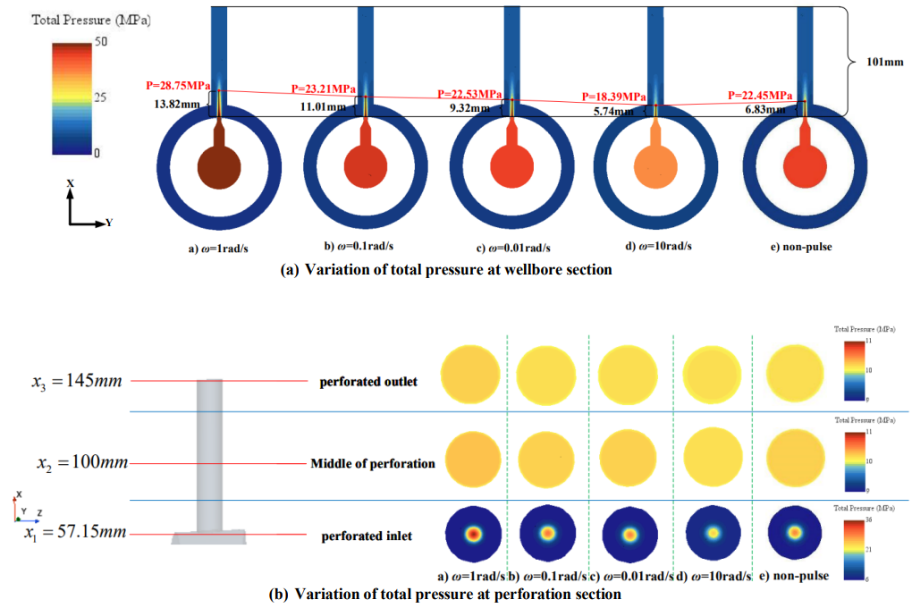
Figure 11: The influence of angular velocity on total pressure at wellbore and perforation section. (Pm=15MPa; P0=45MPa; d=4mm; Dp=15mm) It is necessary to explore the variation of total pressure along the X axis under different angular velocity (Figure 12). According to Figure 12, when the angular velocity is 1 rad/s and 10rad/s, the maximum and lowest total pressures are
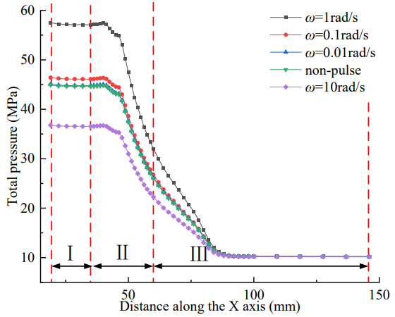
determined to be 57.51MPa and 36.77MPa, respectively. In addition, the overall pressure was lowered by 56.4%. As a result, we may conclude that the greatest total pressure can be obtained by varying the angular velocity.
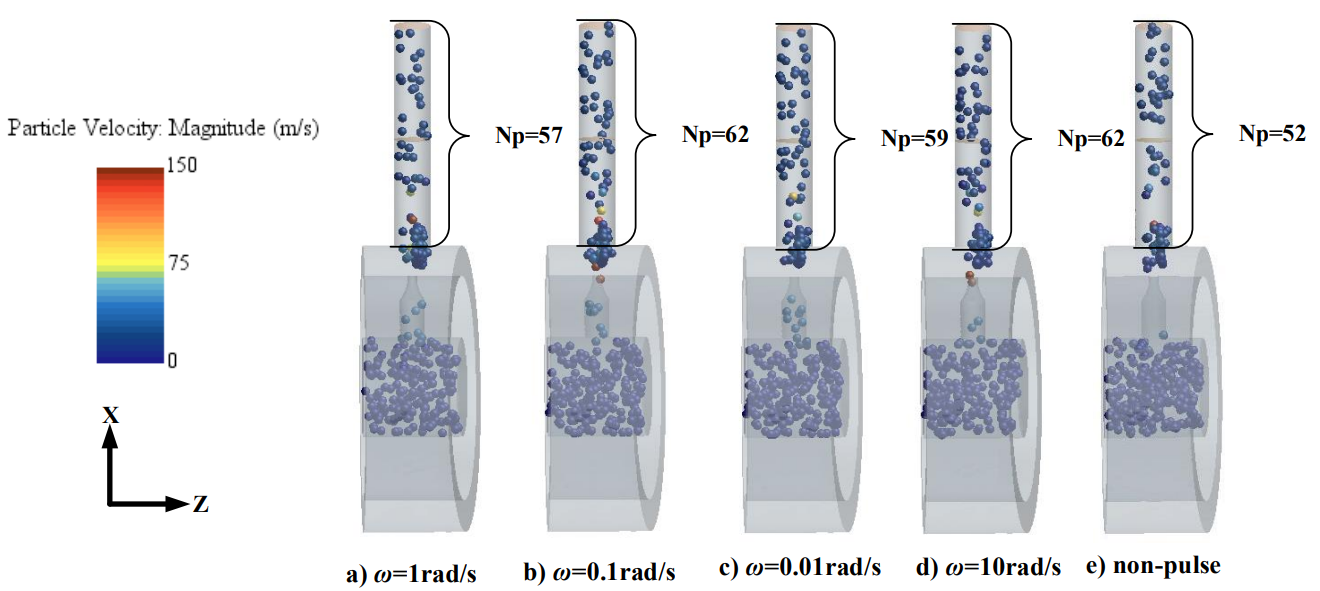
Proppants Transport in The SPJFM: Figure 13 depicts the transit of proppants in the SPJFM at various angular velocity. When the findings for various angular velocity are compared, it is discovered that there are 57, 62, 59, and
62 proppants entering the perforation, correspondingly. In addition, 19%, 20.67%, 19.67%, and 20.67% of proppants penetrate the perforation, correspondingly. The findings show that there is an ideal angular velocity for getting the most proppants into the SPJFT. At the same time, it is obvious that there is a considerable number of proppants obstructing around the perforation inlet of the SPJFM in the non-pulsed jet fracturing. As a result, the pulse jet fracturing helps to remove the proppants that are clogging the perforation inlet.
Effect of Average Pressure (P0)
The Variation of Jet Velocity (V): The variation of velocity at wellbore section and perforation section under different average pressure can be seen in Figure 14. The results show that with the average pressure increasing from 35MPa to 65MPa, the maximum velocity along jet axis sharply increases. When the maximum total pulse pressure (_P_j) varies from 50MPa to 80MPa, the velocity of jet core reaches a maximum value of rises from 229.9m/s to 308.4m/s.
In Figure 14(a), the jet velocity rises from 114.95m/s to 154.20m/s from 15.47mm to 24.85mm along the X axis, representing the corresponding value of 0.5Vmax at 15.3% and 24.6% of the total jet length, respectively. We can see the maximum jet velocity increases with the average pressure increasing. Compared the pulse jet and non-pulse jet, it is shown that when the average pressure _P_0 is 45MPa, the jet velocity of different perforated positions in SPJFT is greater than non-pulsed under the same average pressure.
As can be seen from Figure 15, it is shown the variation of jet velocity along the X-axis to various distance under different average pressure. As the average pressure increases, the pulse jet’s maximum velocity can be achieved and increases gradually. It is found that when the pulse pressure increases from 50 MPa to 80 MPa, the maximum
velocity amplitude increases from 229.9 m/s to 308.4 m/s, an increase of 34.1% in the maximum velocity amplitude. Under the same average pressure, the pulsed case has a faster maximum velocity decrease than the non-pulsed case, which is beneficial to reduce the proppants blocking at the inlet of perforation.
The Variation of Total Pressure (P): It can be seen through Figure 16 that the variation of total pressure at wellbore section and perforation section under different average pressure. As the average pressure increases, the maximum total pressure along jet axis rapidly increases. When the pulse pressure increases from 50MPa to 80MPa, the total pressure of jet core reaches a maximum value varied from 47.5MPa to 77.5MPa. The total pressure is 23.75MPa at 10.94mm and 38.75MPa at 18.71mm along the jet axis, respectively, equivalent to the 0.5_P_max at 10.83% and 18.52% of the entire jet length. Simultaneously, according to the color map in Figure 16(a), the maximum total pressure of the jet from the perforation inlet to the perforation outlet along the jet axis decline gradually under the same average pressure. Also, it can be seen that the maximum total pressure of the jet increases as the intermediate pressure increases. At a moderate pressure of 45MPa, the total pressure at different perforation locations is greater than the non-pulsed case at the same parameter setting.
Figure 16: Variation of total pressure at wellbore section and perforation section under different average pressure. (Pm=15MPa; ω=1rad/s; d=4mm; Dp=15mm) Figure 17 depicts the change of total pressure along the X-axis under various average pressures to examine the impact of average pressure on total pressure. When the pulse pressure climbs from 50MPa to 80MPa, the maximum total pressure rises from 47.5MPa to 77.5MPa, representing a 63.2% increase in maximum total pressure. When the average pressure is 45 MPa, the maximum total pressure in the pulsed scenario is 57.5 MPa. The non-pulsed case, on the other hand, is 44.9MPa, which is 28.7% less than the pulse jet fracturing. As a result, even if the end total pressure is 10MPa, the pulse jet fracturing might produce a higher maximum total pressure in the hole. In other words, as the average pressure rises, so does the maximum total pressure of the jet, resulting in a positive contribution to fracture pressurization in the hole.
Proppants Transport in the SPJFM
As can be seen from Figure 18, it shows the proppants transport in the SPJFM under different average pressure. When the number of proppants carrying under different average pressure are compared, it is clear that there are 66, 57, 64 and 72 at pulse pressures of 50MPa, 60MPa, 70MPa and 80MPa, respectively. And the proportion of proppants entering the perforation is 22%, 19%, 21.3% and 24%, respectively. We can find that the transporting proppants would first decrease and then increase with the average pressure rising. As a compared group, it is worth noting that 52 proppants, 16.67% of total proppants, transport into the perforation under non-pulsed pressure jet. It is found that the number of blocking proppants at the perforation inlet of non-pulse jet fracturing is greater than that of pulsed case jet fracturing, showing that the pulse jet could alleviate proppants blocking in the perforation entrance section.
Effect Of Nozzle Diameter (D)
The Variation Of Jet Velocity (V): It can be seen through Figure 19 that the variation of velocity at wellbore section and perforation section under different nozzle diameter. It is shown that the maximum velocity of the jet at the nozzle outlet increase with the increasing nozzle diameter. When the nozzle diameter is 4mm, the jet core reaches a maximum of 258.7m/s and when the nozzle diameter is 0.5mm, the jet core reaches a maximum of 118.72m/s. It is pointed out that the jet velocity is 129.35m/s at 19.65% jet length when the nozzle diameter is 4mm, equivalent to 0.5_V_max. Also, when the nozzle diameter is 0.5mm, the jet velocity is 59.36m/s, which is equivalent to 0.5_V_max at the position of 0% jet length. It is concluded that when the nozzle diameter is 4mm, the maximum velocity of the jet reduces more rapidly from Figure 19(a). It can be seen that the maximum velocity of the jet increases as the nozzle diameter increases when it is the different parameter. When the nozzle diameter is 4mm, the maximum jet velocity of different perforated parts is greater than the non-pulsed case under the same parameter and the velocity at the perforation outlet is same.
Figure 19: Variation of velocity at wellbore section and perforation section under different nozzle diameter. (Pm=15MPa; ω=1rad/s; P0=45MPa; Dp=15mm) Figure 20 shows the variation of jet velocity along the X-axis to various distances under different nozzle diameters. With the nozzle diameter increasing, the maximum velocity of the pulse jet gradually increases. When the nozzle diameter increases from 0.5mm to 4mm, the maximum velocity increases from 59.36m/s to 129.35m/s, an increase of 117.9% in the maximum velocity. The maximum velocity
decay trend in the pulsed case is greater than in the non- pulsed case under the same nozzle diameter. Consequently, we can conclude that the larger the nozzle diameter, the greater the initial jet velocity from the SPJFT axis and the greater the jet velocity to the nozzle outlet and perforation outlet.
The Variation of Total Pressure (P): The fluctuation of total pressure at the wellbore and perforation sections with varying nozzle diameters, as shown in Figure 21. It can be shown that when the nozzle diameter is less than 4mm, the maximum total pressure of the jet at the nozzle outlet rises as the nozzle diameter grows. When the nozzle diameter rises from 0.5mm to 2mm, maximum total pressure of the jet core varies from 57.62MPa to 57.76MPa. It is noted that the total pressure is 28.81MPa at -2.53mm of the jet axis and 28.88MPa at 2.96mm of the jet axis, respectively, which corresponds to the 0.5_P_max at -2.5% and 2.93% of the total jet length, respectively. Compared with other nozzle diameters, when the nozzle diameter is 4mm, the total pressure is 28.75MPa at 13.82mm of the jet axis, which is equivalent to 0.5_P_max at the position of 13.68% of the entire jet section. When the nozzle diameters are 0.5mm, 1mm and 2mm, respectively, the total pressure changes slightly. When the nozzle diameter is 4mm, the total pressure of the jet in different perforation section is greater than the non-pulsed case under the same nozzle diameter. It can be inferred that the maximum total pressure rises with the increasing nozzle diameter at the nozzle outlet.
Figure 21: Variation of total pressure at wellbore section and perforation section under different nozzle diameter. (Pm=15MPa; ω=1rad/s; P0=45MPa; Dp=15mm) As can be seen in Figure 22, it shows the variation of total pressure along the X-axis to various distances under different nozzle diameters. When the nozzle diameter increases from 0.5mm to 2mm, the maximum total pressure increases from 57.62MPa to 57.76MPa, the maximum total pressure increases by 0.24%. When the nozzle diameter is 4mm, the maximum total pressure that can be achieved in the pulse case is 57.5MPa, and the maximum total pressure of non- pulse case is 44.9MPa, which has a large gap of 28.06% of the maximum total pressure. It can be observed that the smaller the nozzle diameter, the earlier and faster the total pressure reduce. The pulsed case decreases faster than the non-pulsed case when the nozzle diameter remains constant.
Proppants Transport in the SPJFM: It shows the comparison of the proppants transport in the SPJFM under different nozzle diameters in Figure 23. In the pulsed jet case, when the nozzle diameters are 0.5mm, 1mm, 2mm and 4mm, respectively, the number of proppants entering the perforation are 0, 89, 202 and 57, and the ratio of proppants entering the perforation is 0, 6.15%, 21.7% and 19%. As the diameter of the nozzle increases, the proportion of proppants entering the perforation first increases and then decreases.
In the non-pulsed case, with a nozzle diameter of 4 mm, the number of proppants entering the perforation is 52 and the proportion of proppants entering the perforation is 16.67%. It can be seen that the non-pulsed jet fracturing delivers more blocking proppants at the perforation inlet than pulsed case jet fracturing does. When the proppants are of a certain size and the nozzle diameter is very small, it is difficult for the proppants to enter the perforation.
Effect of Perforation Diameter (Dp)
The Variation of Jet Velocity (V): Figure 24 shows the variation of velocity at wellbore section and perforation section under different perforation diameters. When the perforation diameter is 10mm, the jet core reaches a maximum velocity of 277.08m/s; When the perforation diameter is 25mm, the jet core reaches a maximum velocity of 249.16m/s. The jet velocity is 138.54m/s when the perforation diameter is 10mm, which is equivalent to 0.5_V_max at the position of 14.7% jet length, measured at 14.85mm along the jet axis. And when the perforation diameter is 25mm, the jet velocity is 124.58m/s, which is equivalent to 0.5_V_max at the position of 18.4% jet length, measured at 18.55mm along the jet axis. With a perforation diameter of 10 mm, the maximum velocity of the jet decreases more rapidly.
Figure 24: Variation of velocity at wellbore section and perforation section under different perforation diameter. (Pm=15MPa; ω=1rad/s; P0=45MPa; d=4mm) When the perforation diameter is 15mm, the maximum jet velocity of the various perforation sections is greater than that of the non-pulsed case with the same perforation diameter. Finally, it is concluded that the maximum velocity of the jet gradually decreases as the perforation diameter increases.
Figure 25 displays the variation of jet velocity along the X-axis to various distances under different perforation diameters. The maximum velocity of pulse jet is different from another perforation diameter. When the perforation diameter varied from 10mm to 25mm, the maximum velocity decreased from 277.08m/s to 249.16m/s, and the maximum velocity reduced by 11.21%. It can be found that when the diameter of the perforation is larger than 10mm, there is a smaller value of the maximum velocity than in other cases. When the perforation diameter remains constant, the velocity of the pulsed case reduces faster than that of the non-pulsed case.
The Variation of Total Pressure (P): In Figure 26, there is the variation of total pressure at wellbore section and perforation section under different perforation diameters. When the perforation diameter is 15mm, the jet core reaches a maximum total pressure of 57.5MPa. It is pointed out that the total pressure is 28.75MPa at 13.82mm along the jet axis, which corresponds to the 0.5_P_max at 13.68% of the total jet length. And when the perforation diameter is 10mm, the total pressure is 28.57MPa at 9.28 mm along the jet axis, which is an equivalent value of 0.5_P_max at the position of 9.2% jet length. Under non-pulsed pressure, when the perforation diameter is 15mm, the total pressure of the jet core is 22.45MPa, and the length is 6.83mm, which is equivalent to the 0.5_P_max at 6.76% of the entire jet length.
Figure 26: Variation of total pressure at wellbore section and perforation section under different perforation diameter. (Pm=15MPa; ω=1rad/s; P0=45MPa; d=4mm) When the perforation diameter is 15mm, the total pressure of the jet in different perforation sections under the pulsed condition is greater than the non-pulsed case with the same parameter setting. In the case of pulse jet, the change of the perforation diameter has little effect on the maximum total pressure of the jet at the nozzle outlet, and the degree of change in the total pressure is small.
Figure 27 shows the variation of total pressure along
the X-axis to various distances under different perforation diameters. Among them, when the perforation diameter is varied from 10mm to 15mm, the maximum total pressure increases from 57.14MPa to 57.5 MPa, and the maximum total pressure increases by 0.63%. It can be obtained that the smaller the perforation diameter, the earlier and faster the reduction of the total pressure. When the perforation diameter is fixed, the total pressure in the pulsed case decreases faster than in the non-pulsed case.
Proppants Transport in the SPJFM: As shown in Figure 28, there is the comparison of the proppants transport in the SPJFM under different perforation diameters. The number of proppants entering the perforation under pulse conditions are 21, 57, 103, and 126, respectively, and the proportion of proppant entering the perforation is 7.29%, 19%, 31.12%, and 33.24% for perforations with diameters of 10mm, 15mm, 20mm, and 25mm, respectively. When the perforation diameter is 15mm in the non-pulsed case, the number of proppants entering the perforation is 52, and the proportion of proppants entering the perforation is 16.67%. It can be found that as the diameter of the perforation increases, the number of proppants entering the perforation also increases. Simultaneously, when all other parameters are maintained, the smaller the diameter of the perforation, the less proppant enters the perforation, and some of the proppant appears in the annular section.
Conclusions
In this paper, a single section of pulse jet fracturing model (SPJFM) was established through the CFD/DEM coupling method to explore the pressurization characteristics and proppants transport of pulse jet fracturing. The effects of pressure amplitude, angular velocity, average pressure, nozzle diameter and perforation diameter on the jet and proppants transport in the SPJFM were discussed, and the following conclusions are obtained:
- Under the effect of different parameters, the maximum velocity and maximum total pressure that can be achieved by the pulsed jet are different. Among them, the effect of parameters such as pressure amplitude and average pressure was positively correlated with the maximum velocity and maximum total pressure. The effect of nozzle diameter was positively correlated with the maximum velocity, and the maximum total pressure has a relatively small effect. The effect of perforation diameter is negatively correlated with the maximum velocity, and the influence on the maximum total pressure is less. There are optimal parameters for the effect of angular velocity, that is, when the angular velocity ω=1rad/s, the maximum jet velocity and the maximum total pressure are obtained.
- Depending on the effect of different parameters, the number and proportion of proppants entering the perforation through the jet are different.
Under the same conditions, the amount of proppant entering the perforation in the case of a pulsed jet is 57, while the non-pulsed jet is only
Acknowledgments
The authors express their appreciation to the National Natural Science Foundation of China (Grant No.52004236), the Key Program of National Natural Science Foundation of China (Grant No. 52234003), the Open Project Program of Engineering Research Center of Geothermal Resources Development Technology and Equipment, Ministry of Education (Grant No.22016), the Open Project Program of Panzhihua Key Laboratory of Advanced Manufacturing Technology (Grant No. 2022XJYB01), Open Fund (PLN 2022-37 ) of State Key Laboratory of Oil and Gas Reservoir Geology and Exploitation (Southwest Petroleum University), the Starting Project of SWPU (Grant No.2019QHZ009), and the Chinese Scholarship Council (CSC) funding (CSC NO.202008515107).
References
-
Hu W, Zhai G, Li J (2010) Potential and development of unconventional oil and gas in China. Strategic Study of CAE 12(5): 25-63.
-
Ma F, Sang Y (2008) Optimization of key parameters of coiled tubing hydraulic injection fracturing. Natural Gas Industry (1): 76-78.
-
Tian S, Li G, Huang Z, Niu J, Xia Q (2008) Coiled tubing hydraulic injection fracturing technology. Natural Gas Industry (8): 61-63.
-
Wang T, Xu Y, Jiang J, Tian Z, Ding Y (2010) Coiled tubing hydraulic jet annulus fracturing technology. Natural Gas Industry 30(1): 65-67.
-
Qu H, Li G, Huang Z, Tian S (2010) Internal pressurization mechanism of hydraulic jet fracturing bore. Journal of China University of Petroleum 34 (5): 73-76.
-
Qu H, Li G, Huang Z, Li X, Zhao W, et al. (2011) Hydraulic jet fracturing seal mechanism. Acta Petrolei Sinica 32(3): 514-517.
-
Qu H, Li G, Liu Y, Sheng M, Chun W (2012) Study on sealing pressure field of hydraulic injection fracturing jet. Fluid Machinery 40(11): 21-24.
-
Zhang J (2015) Study on hydraulic jet fracturing parameters. Southwest Petroleum University, China.
-
Fan X, Li G, Huang Z, Niu J, Song X, et al. (2015) Full- scale experiment of air hydraulic isolation in hydraulic jet fracturing. Journal of China University of Petroleum 39(2): 69-74.
-
Xia Q, Huang Z, Li G, Zhao Z, Fu G, et al. (2009) Experimental study on the law of jet pressurization in hydraulic injection hole. Fluid Machinery 37(2): 1-5.
-
Sheng M, Li G, Huang Z, Tian S, Qu H, et al. (2011) Numerical simulation of jet pressurization law in hydraulic injection hole. Drilling & Production Technology 34(2): 42-45.
-
Chen C, Meng Y, Zhong X, Nie S, Ma Y, et al. (2021) Research on the Influence of Injection-Production Parameters on Challenging Natural Gas Hydrate Exploitation Using Depressurization Combined with Thermal Injection Stimulated by Hydraulic Fracturing. Energy & Fuels 35(19): 15589-15606.
-
Ge Z, Zhang H, Zhou Z, Cao S, Zhang D, et al. (2023) Experimental study on the characteristics and mechanism of high-pressure water jet fracturing in high- temperature hard rocks. Energy 270.
-
Xue Y, Si H, Hu Q (2017) The propagation of stress waves in rock impacted by a pulsed water jet. Powder Technology 320: 179-190.
-
Cai C, Kang Y, Wang X, Hu Y, Huang M, et al. (2019) Experimental study on shale fracturing enhancement by using multi-times pulse supercritical carbon dioxide (SC- CO2) jet. Journal of Petroleum Science and Engineering 178: 948-963.
-
Cheng Z, Xu Y, Xiang X, Li Q, Wu S, et al. (2015) Experimental study of pulsating water pressure propagation in CBM reservoirs during pulse hydraulic fracturing. Journal of Natural Gas Science and Engineering 25: 15-22.
-
Zhang H, Huang Z, Li G, Lu P, Tian S, et al. (2018) Fracture propagation and acoustic emission response characteristics of radial well-pulsating hydraulic fracturing in coal rock. Acta Petrolei Sinica 39(4): 472- 481.
-
Liu Y, Mu S, Guo J, Li Q, Hu D, et al. (2022) Analytical model for fracture conductivity considering rod proppant in pulse fracturing. Journal of Petroleum Science and Engineering 217: 110904.
-
Lu P, Li G, Shen Z, Huang Z, Sheng M, et al. (2015) Numerical simulation of stress disturbance effect of fracture filling on pulsating hydraulic fracturing. Journal of China University of Petroleum 39(4): 77-84.
-
Lu P, Li G, Huang Z, Song X, Sheng M (2015) Numerical model and solution of dynamic and static response of pulsating hydraulic fracturing of coal seam. Rock and Soil Mechanics 36(5): 1471-1480.
-
Liao S, Hu J, Zhang Y (2022) Investigation on the influence of multiple fracture interference on hydraulic fracture propagation in tight reservoirs. Journal of Petroleum Science and Engineering 211: 110160.
-
Dehkhoda S, Hood M (2013) An experimental study of surface and sub-surface damage in pulsed water- jet breakage of rocks. International Journal of Rock Mechanics and Mining Sciences 63: 138-147.
-
Liu Y, Wei J, Ren T, Lu Z (2015) Experimental study of flow field structure of interrupted pulsed water jet and breakage of hard rock. International Journal of Rock Mechanics and Mining Sciences 78: 253-261.
-
Wang Z, Kang Y, Xie F, Shi H, Wu N, et al. (2022) Experimental investigation on the penetration characteristics of low-frequency impact of pulsed water jet. Wear 488-489.
-
Zhang Y, Long H, Tang J, Ling Y (2023) Experimental Investigation on the Granite Erosion Characteristics of a Variable Cross-Section Squeezed Pulsed Water Jet. Applied Sciences 13(9): 5393.
-
Hari S, Krishna S, Gurrala L, Singh S, Ranjan N, et al. (2021) Impact of reservoir, fracturing fluid and proppant characteristics on proppant crushing and embedment in sandstone formations. Journal of Natural Gas Science and Engineering 95: 104187.
-
Zhao J, Shan T (2013) Coupled CFD-DEM simulation of fluid-particle interaction in geomechanics. Powder Technology 239: 248-258.
-
Li H, Lee A, Fan J, Yeoh G, Wang J (2014) On DEM-CFD study of the dynamic characteristics of high speed micro- abrasive air jet. Powder Technology 267: 161-179.
-
Zhu H, Shen J, Zhou H (2018) Numerical simulation of propped fracture conductivity. Acta Petrolei Sinica 39(12): 1410-1420.
-
Guo T, Gong Y, Liu X, Wang Z, Xu J, et al. (2022) Numerical simulation of proppant transport and placement in complex fractures. Journal of China University of Petroleum 46(3): 89-95.
-
Cai C, Gao C, Wang H, Pu Z, Tan Z, et al. (2021) High- pressure CO2 jet-PDC tooth composite rock-breaking flow field and rock carrying enhancement mechanism. Natural Gas Industry 41(10): 101-108.
-
Qu H, Li G, Huang Z, Liu Z, Shi M (2011) Study on pressure distribution in hydraulic jet pressure hole. Journal of Southwest Petroleum University 33(4): 85-88.
-
Cheng Y, Li G, Wang H, Shen Z, Tian S (2014) Flow field characteristics in supercritical CO2 jet fracturing holes. Journal of China University of Petroleum 38(4): 81-86.
-
Shi H, Li G, Huang Z, Li J, Zhang Y (2015) Study and application of a high-pressure water jet multi-functional flow test system. Rev Sci Instrum 86(12): 125111.
- Nigeria’s Vulnerability in the Face of Global Energy Policy
- A Simulation Study of Investigation of Optimum Oil Production Performance by Applying Various Gas Injection Methods in Oil Reservoir
- Characterization of Permo-Triassic Reservoirs through Thermal Maturity Assessment of Westphalian Source Rocks in the Cheshire Basin
- Influence of Microwax on the Rheological and Thermal Behaviour of a Wax Crude Oil
- Real-Time Monitoring and Performance Optimization of Steam Injection in Heavy Oil Reservoirs Using Fiber Optic Sensing and Integrated Predictive Simulation Models
- Rapid On-Site Determination of the Total Petroleum Hydrocarbon Content of Soils by Handheld Fourier Transform Near-Infrared Spectroscopy: Development of a Global, Site- and Scanner- Independent Calibration Model