
Many Discrete Worlds
We present the case for a fixed, finite number of discrete, non-interacting, spatiotemporally finite, decohered spacetimes emerging from Everett’s Universal Wave Function, which we refer to as “Many Discrete Worlds” (MDW). No universes “split” in MDW. We argue that a Many Worlds Interpretation (MWI) branching structure that emerges after decoherence is equivalent to individual, weighted universes, each of which is divided into an immense number of discrete, identical copies, the number being proportional to the individual weighting. This ensures that repeated experiments within any such universe will demonstrate consistency with the Born rule. Each of these universes should be considered as complete, containing every decohered outcome over the entire extent of its spacetime, including every event/interaction occurring beyond any cosmological particle horizon for the entire duration of the given universe. We show that a countably infinite number of interactions needs an uncountably infinite number of universes, and show why measures such as the Lebesgue measure will fail in that case, with the result that the Born rule would not be demonstrable. This leads to the conclusion that the number of universes in the multiverse must be finite and, as a surprising corollary, that the universes themselves are finite, both in space and duration.
Introduction
Of the dozen or so mainstream interpretations of quantum mechanics, each with its own many variants (for a list of the most important ones, see e.g., Freire, et al. [1]), Hugh Everett’s Many Worlds Interpretation (MWI) (Everett [2]) has attracted perhaps more than its share of controversy and debate. (For an excellent introduction to the whole debate, see the book edited by Saunders, et al. [3] and Saunders’ own introduction to the book (Saunders [4]) as well as many other papers including, for example, Kent [5, 6], Butterfield [7, 8], Hartle [9], Greaves and Myrvold [10], Zurek [11], Barrett [12], Tappenden [13, 14, 15], Adlam [16], Papineau and Rowe [17], Vaidman [18].). The purpose of our paper is to argue the case for a subset of MWI where our universe is one of an unimaginably large but nevertheless finite number of discrete, non-interacting, decohered Minkowski spacetimes distributed in proportion to the Born Conceptual probabilities of the quantum outcomes embedded within each of those spacetimes. This means that there are generally multiple identical copies of any given spacetime/universe/ world. We shall go on to argue that, counterintuitively, all of these universes are finite, both spatially and temporally. For brevity we refer to this picture as Many Discrete Worlds (MDW).
Decohered Histories
Our point of departure is to consider the history of our universe viewed from an arbitrary world line. This history will be defined by a series of outcomes of quantum events along the chosen world line, where, by an “event”, we mean what is often called a “measurement” but is really any interaction that results in a change of state such as a change in electron spin or momentum. These events do not generally happen directly on the world line but originate instead from anywhere within the universe: the arrival of the light cone from such a distant event impinging upon the world line might be considered as marking a corresponding branching point on the world line. (The concept of the light cone signalling such a “collapse” is not new—see, for example, Belnap [19], Bacciagaluppi [20] or Figure 8.2 of Wallace’s book (Wallace [21])—but decoherence is sometimes considered to spread out at subluminal velocities: e.g. Marvian and Lidar [22]. For our purposes, it doesn’t matter which we choose.) To make this concrete, consider Figure 1, adapted from Figure 3 of Hartle’s [23] pedagogical introduction to a “coarse-grained” picture (in effect, after decoherence is complete)—a picture that was further developed by Gell- Mann and Hartle [24]. The figure shows a wave function, ψ , expressed as the branching structure of a set of 16 alternative histories (i.e., branches), each containing three events/interactions marked by black dots. In our adaptation, we assume that the three events are mutually independent, which was unnecessary in Hartle’s example. One particular branch is highlighted with a heavier line, but in each of the 16 branches, the three events have already occurred, so that no quantum interference is explicitly portrayed in the figure—the branches are completely decohered. Any evidence of interference would only be manifest in patterns involving the alternative outcomes themselves: for example, interaction #3 has four different possible outcomes. If these four outcomes are regarded for instance as a schematic of four possible regions where an electron might land on a detecting screen after encountering a double slit, then the relative probabilities of each of the four outcomes would be a manifestation of the interference.
These branches are generally regarded as worlds or universes. While Boughn [25] and others remind us that Everett [2] himself spoke of states branching, other authors such as Wallace ([21], pp: 63), spoke of the branches being “not any less real”, a view endorsed over time by authors including DeWitt [26], Vaidman [27], Wilson [28], Hall, et al. [29]; even Everett agreed that “It looks like we would have a non-denumerable infinity of worlds” (Werner [30], pp: 95 marked “Tuesday am page 20”).
![Figure 1: This figure, adapted from Hartle [23], shows the branching structure of a set of 16 alternative histories that constitute the wave function ψ , featuring three interactions. The probability amplitude associated with each interaction is _α__nk_, where _n_ refers to interaction #_n_ and _k_ is the _k_th alternative outcome for that interaction. Thus, ψ is the superposition of the 16 histories, each history being the tensor product of the three vectors _nk_ ψ associated with the three interactions. One of the 16 alternative branches has been highlighted for discussion in the text.](/fulltextimages/14237/fig_1.png)
Figure 1: This figure, adapted from Hartle [23], shows the branching structure of a set of 16 alternative histories that constitute the wave function ψ , featuring three interactions. The probability amplitude associated with each interaction is αnk, where n refers to interaction #n and k is the k_th alternative outcome for that interaction. Thus, ψ is the superposition of the 16 histories, each history being the tensor product of the three vectors _nk ψ associated with the three interactions. One of the 16 alternative branches has been highlighted for discussion in the text.
The probability amplitude associated with each interaction in Figure 1 is αnk, where n refers to interaction #n and k is the _k_th alternative outcome for that interaction (so that, in our figure, there are four alternative outcomes for interaction #3). Following Gell-Mann and Hartle [24], the branch probability of the highlighted branch—effectively, the probability of finding yourself in a universe represented by this particular
The Frequency Distribution of Universes in MDW
branch—is:
prob. of being in universe 112232 ψ = 2 2 2 2 11 22 32 11 22 32 . . . . α α α α α α = (1) where we have used 112232 ψ for the highlighted branch.
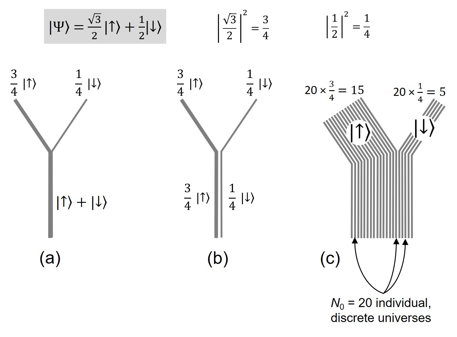
Figure 2: The branching for the two outcomes of the 60º Stern-Gerlach experiment described in the text is shown in (a), with weightings according to the absolute squares of the probability amplitudes. The equivalent divergent/discrete picture is shown as two separate, weighted universes in (b). In (c), each of these two weighted universes is divided into multiple identical copies in numbers proportional to the weights.
In this section we propose a frequency distribution for the parallel universes over the whole MDW multiverse, which will be based on the Born rule. We go on to show, in the following section, how this distribution will lead to experimental results in any one universe which are indeed consistent with the Born rule. Note that we are not attempting to derive the Born rule here: we accept it as a given.
Consider an experiment where a particle with a vertically upward spin passes through a Stern-Gerlach magnet inclined at 60º to the vertical. The state of the particle just before it is detected may be written as 3 1 2 2 ↑+ ↓, where the spins in states ↑ and ↓ are inclined at 60º to the vertical, in alignment with the Stern-Gerlach detector; call them “spin- up” and “spin-down” respectively. Figure 2 shows the branching structure for the experiment. Figures 2(a) and 2(b) follow Figure 1(a) and Figure 1(c) of Saunders [31], who shows how the branching (or “overlapping”) and discrete (or “divergent”) pictures are equivalent. The weights of the branches are the Born probabilities for the outcomes and $|\downarrow\rangle$, namely $\frac{3}{4}$ and $\frac{1}{4}$ respectively. (For further discussion of weighted branching, see, for instance, Lewis [32], Saunders and Wallace [33], Saunders [4], Wallace [21], Wilson [34], Tappenden [15]).
To address the problem of why an observer should give more credence to being in a universe with a greater weight, we use the "branch counting" method employed in different ways by several authors: to a given universe, we assign a number of equally weighted universes in proportion to its branch weight—see, for instance, Khawaja [35], Saunders [36], and Barrett and Goldbring [37], with the latter authors using a model based on nonstandard analysis, which, in the opinion of Khawaja, may be compatible with branch counting.
Wallace [21] asks how branches can be counted when, in his words, "there is actually no such thing as the number of branches". The main issue is the preferred basis—if any rotated basis is equally valid, how can we fix on any particular basis for counting the branches? Should our summation even include the branches in all of the other possible bases? Our approach to these questions is to consider the branches only after the interactions have completely decohered—in that case, whatever it was in the environment that selected the particular basis for the observed outcome, that same process rules out all of the putative alternative bases.
In Figure 2(c) we have replaced each of the two single, weighted branches by discrete universes in numbers proportional to the weights, identical to each other within a given branch. For the illustration we have assumed that the $60^\circ$ experiment is the only event in the universe and that there are only 20 discrete universes in the multiverse. At first glance, Figure 2(c) looks as though it might represent Saunders' equi-amplitude branch-counting picture (Saunders [36]), but that would be too quick. While it is true that branch-counting in Saunders' scheme results in numbers proportional to the squares of the histories' probability amplitudes, his approach is more subtle than ours in that it accounts for all possible branch histories, whereas ours is a considerably blunter instrument, selecting only the final, completely decohered history. So, the many universes in Figure 2(c) are identical copies of either the single state (the left branch), or the single state (the right branch). Furthermore, we are not trying to derive the Born rule in any way—in MDW we simply accept that an outcome of the universal wave function is that, at complete decoherence, at the extreme coarse-grained level, there are multiple identical copies of universes in numbers proportional their respective Born probabilities.
The number of discrete, decohered universes in the multiverse, $N_0$, is fixed—and also finite, as we shall argue later—and the occurrence of an event does not mean that the number of universes increases to contain the event's outcomes. The distribution of these universes is tenseless and determinate. Each universe is discrete and doesn't split: they are simply part of the structure of the multiverse. Note also that the fixed number of universes means that the MDW multiverse is not amenable to analysis such as that applied by Short [38] to discrete many-worlds models, where his analysis exposes contradictory values for probabilities$^1$.
As we shall discuss in more detail in (Section: Spatiotemporally Finite Universes in a Finite Multiverse), the number of events in the multiverse cannot be greater than the number of universes, $N_0$, needed to contain all of the different outcomes of each of these events. Since $N_0$ is finite, we can identify individual events with a label, $n$. Of course, no universe in the multiverse will contain every event: the configurations of individual universes—meaning the complete history of all of the event outcomes that the universes contain, along with the spacetime locations of the outcomes from beginning to end—are determined by the unitarily evolving state from which the complete decohered history may in principle be extracted. We shall use $N_0$ for the number of events in the $n^{\text{th}}$ universe with a given configuration of outcomes. Since a given universe/branch can contain only one outcome of the $n^{\text{th}}$ event, then the number of different universes containing a specific event has to be at least as great as the total number of possible outcomes of that event. For a given event, a list of the different possible outcomes may be found within the sum of the vectors for all possible outcomes of the event:
$$\sum_{k_n} |\psi_{ink_n}|$$
where $k_n$ is the $k^{\text{th}}$ outcome of the $n^{\text{th}}$ event in the $i$th universe.
1 In effect, Short considers a multiverse containing two universes, $|0\rangle + |1\rangle$ so that the probability of being in either one is $\frac{1}{2}$. Then he applies a transformation that transforms $|1\rangle$ into $|1\rangle + |2\rangle$, leaving the $|0\rangle$ intact, so that there are now three universes, $|0\rangle + |1\rangle + |2\rangle$. By the axioms in the paper, this means that the probability of being in any one of the final three universes is $\frac{1}{4}$, which is a contradiction. However, in MDW, there is no contradiction, and in this scenario there would be four universes at the outset, $|0_1\rangle + |0_2\rangle + |1_1\rangle + |1_2\rangle$, with a probability of $\frac{1}{4}$ of being in any one, making a total probability of $\frac{1}{4}$ of being in $|0\rangle$, or $|1_2\rangle$, are still $\frac{1}{4}$, $\frac{1}{4}$, and $\frac{1}{4}$ respectively, and there is no contradiction.
For illustration, the sum of the two possible outcomes for interaction #1 in Figure 1 would be
$$\left( |\psi_{i11}| + |\psi_{i12}| \right)$$
where “$1$” and “$2$” refer to the outcomes represented by $\alpha_{11}$ and $\alpha_{12}$, respectively in Figure 1 (and, for instance, “$2$” and “$2$” would refer the outcomes of the event in state $|\psi_{i2}|$ represented by $\alpha_{21}$ and $\alpha_{22}$ respectively).
The complete state for any universe in the multiverse may be found as a unique branch within the collection of all possible combinations of the outcomes of all $N_i$ events contained in each branch, where the product sign is to be understood as the tensor product:
$$\prod_{n=1}^{N_i} \sum_{k_i} |\psi_{i n k_i}|$$
Remember that the events with their outcomes are assumed here to be unentangled, i.e., independent. As we shall discuss in (Section: Entanglement in MDW), entangled events are considered as a single event, but the arithmetic doesn’t change otherwise.
Using (2), and continuing with the same illustration, the collection of all possible combinations of the outcomes of interactions #1 and #2 in a given universe, $i$, where there are no other events, is:
$$\left( |\psi_{i11}| + |\psi_{i12}| \right) \otimes \left( |\psi_{i21}| + |\psi_{i22}| \right)$$
$$= |\psi_{i11}| |\psi_{i21}| + |\psi_{i11}| |\psi_{i22}| + |\psi_{i12}| |\psi_{i21}| + |\psi_{i12}| |\psi_{i22}|$$
where the tensor product sign has been dropped. These represent the four possible branches in Figure 1 containing interactions #1 and #2.
As we mentioned, not every event in the multiverse appears in every universe. For instance, suppose that an event described by a state $|\psi_{i4k}|$ is triggered by the interaction #1, but only if the outcome is $|\psi_{i11}|$ and not $|\psi_{i12}|$, so that, in universes where the outcome is $|\psi_{i12}|$, there is no state $|\psi_{i4k}|$. If there are three possible outcomes to the event in state $|\psi_{i4k}|$, written $|\psi_{i41}|$, $|\psi_{i42}|$, $|\psi_{i43}|$, then, from (2), there are 8 possible configurations of universes, as shown by the following combinations of vectors:
$$|\psi_{i11}| |\psi_{i21}| |\psi_{i41}| + |\psi_{i11}| |\psi_{i21}| |\psi_{i42}| + |\psi_{i11}| |\psi_{i21}| |\psi_{i43}|$$
$$+ |\psi_{i12}| |\psi_{i21}| |\psi_{i41}| + |\psi_{i11}| |\psi_{i21}| |\psi_{i42}| + |\psi_{i11}| |\psi_{i21}| |\psi_{i43}|$$
where the last two terms do not contain the state $|\psi_{i4k}|$ by the supposition.
We assign a unique identifier to each universe with a given configuration of event outcomes, so that, even although two states for a universe may be otherwise identical, they are nevertheless distinguished by the value of the label, $i$. The number distribution of such universes, identical but for their labels, is determined by the Born rule. The configuration of outcomes in a given universe within the collection of universes in (2) may be specified thus:
$$\prod_{n=1}^{N_i} |\psi_{i n k_i}|$$
where only one outcome for each event $n$ is selected, namely outcome $k_n$. An example would be the triplet of vectors in the second term of (3), namely, $|\psi_{i11}| |\psi_{i21}| |\psi_{i42}|$. In general, the otherwise identical universes with this particular configuration may be distinguished by their label, $i$, as in this expression which uses the summation to allocate a different value of $i$ to each configuration:
$$\sum_{n=1}^{N_i} \prod_{n=1}^{N_i} |\psi_{i n k_i}|$$
where $|\alpha_{nk_i}|^2$ is the absolute square of the probability amplitude for the $k_n$th outcome of event $n$. The upper limit of the sum in (5) is the number of identical universes in the multiverse with the configuration in (4), as derived from the Born rule:
$$N_0 \prod_{n=1}^{N_i} |\alpha_{nk_n}|^2$$
Because we have used the Born rule to arrive at this number distribution, then, as we shall see later, the Born rule re-emerges experimentally within individual universes.
Continuing the illustration, if we assume, say, $\sqrt{\frac{3}{4}}, \frac{1}{\sqrt{2}}$, and $\sqrt{\frac{3}{5}}$ for the probability amplitudes $\alpha_{11}$, $\alpha_{21}$, and $\alpha_{42}$ respectively, then we see from (6) that the number of universes in the multiverse having the above configuration,
$$|\psi_{i11}| |\psi_{i21}| |\psi_{i42}|$$ is:
$$N_0 \prod_{n=1}^{N_i} |\alpha_{nk_n}|^2 = N_0 |\alpha_{11}|^2 |\alpha_{21}|^2 |\alpha_{42}|^2 = 40 \times \frac{3}{4} \times \frac{1}{2} \times \frac{3}{5} = 9$$
where there is no $|\alpha_{3k_n}|^2$ in the product because it doesn’t appear in (3). We have assumed for the illustration that there are just 40 universes in this multiverse, including multiple copies of the possible universes. Of course, nothing subtle is going on here; essentially, all we are saying is that, for a given configuration of outcomes, the number of identical universes in the multiverse with that configuration is proportional to the product of the probabilities of the individual outcomes according to the Born rule.
Now we check that MDW gives the same result as (1) for the probability of the highlighted branch in Figure 1. The probability amplitudes for the outcomes of the three events in the branch are α_11, α22, and α_32 respectively.
Expression (6) gives the number of universes containing these three events with these particular outcomes:
2 2 2
0 11 2 2 3 2 . . N α α α Therefore, the probability of being in such a universe is, trivially,
| N 0 | α 11 | 2 . | α 2 2 | 2 . | α 3 2 | 2 |
|---|
N which, of course, is the same result that we found in equation (1) using the branching model of Gell-Mann and Hartle [24]. It is also in the same format as given by Saunders [36], except that he still grants some uncertainty in the precise numbers of universes because of any residual interference, no matter how small, whereas, in MDW, we are considering the universes only after any interference between event outcomes has been irreversibly wiped out.
Everett’s universal wave function is at the heart of MDW just as it is in MWI and other interpretations of quantum mechanics, and this leads to the same mathematics and the same observed quantum-mechanical outcomes in MDW as in the other interpretations. The agreement between the results of equations (1) and (7) just emphasizes the equivalence of the overlapping picture in Figure 2(a) and the MDW picture in Figure 2(c).
Beyond the Cosmological Particle Horizon
Clearly, in the branching picture, the order of events along a given world line as they are drawn from trunk to twig is schematic, and depends, for instance, on the spatiotemporal locations of the events in relation to the given world-line. In the MDW picture, since the Universal Wave Function is deterministic, each decohered universe contains the outcome of every event from the root event at the beginning to the final event in that universe. Importantly, in MDW, this includes events beyond the cosmological particle horizon: the vectors in (4) include the outcome probabilities of such events. The reasoning goes as follows. Consider a photon reaching Earth as part of the cosmological microwave background, and suppose that the photon is linearly polarized as a result of a Thomson scattering by a free electron during the decoupling phase some 380,000 years after the start of our universe, at a location which is currently just inside our particle horizon, about 46 billion light-years from us. Let ||T be the polarization outcome of the Thomson interaction, with a probability amplitude, α||, and let T⊥ be the state for the alternative outcome, i.e., a perpendicular polarization, with a $$ \left| \alpha_ {\parallel} \right| ^ {2} + \left| \alpha_ {\perp} \right| ^ {2} = 1. $$
. Note that
these probabilities refer to the outcomes of the scattering
interaction, and not the probability of the photon reaching
Earth 13.8 billion years later.
probability amplitude α⊥, where So, there are two weighted universes with distinct configurations: one containing the state TΠ, which happens to be the universe we inhabit, and the other one containing the alternative state T⊥. But that Thomson interaction occurred at a location which was, at that time, because of inflation, beyond our particle horizon: it has only recently come inside it (Davis and Lineweaver [39]). Since there are currently universes with two different configurations, ( TΠ and T⊥), and since discrete universes don’t split in the MDW picture, then the two separate configurations have “always” existed even though the “T” event occurred when it was beyond our particle horizon.
Nevertheless, a belief may still linger that the two configurations of universe only came into existence at the moment when the light cone from the T event reached us (in the form of a cosmological background photon). The counter to that is that we can make the same argument for a photon received from the cosmological microwave background in a diametrically opposite direction in the sky from that in which the TΠ photon reached Earth: let two such states be SΠ and S⊥, where SΠ refers to the polarization outcome in our universe. So, for the two events, there are four configurations of universe, containing, respectively, the states { } T S + Π Π (which is the universe that we inhabit), { } T S⊥ + Π , { } T S ⊥+ Π , and { } T S ⊥ ⊥ + . The key point is that the T event and the S event are separated by some 92 billion light-years, and so are currently beyond each other’s cosmological particle horizon, and yet they nevertheless appear together in four configurations of parallel universe. We could continue this argument by shifting Earth’s point of view to the S event, and then further again, indefinitely across the universe. That is why, in MDW, we include probabilities of all events beyond the particle horizon in expression (4).
Experimental Verification of the Born Rule In MDW
We recognise that such a straightforward notion of probability in equation (7) is frequentist, and may be challenged, particularly as we make the case in Section: Spatiotemporally Finite Universes in a Finite Multiverse that _N_0 is finite. Saunders [31, 40] analyses the fundamentals of probability in quantum mechanics, and self-locating uncertainty is discussed by many authors, often as an adjunct to deriving the Born rule (see, for instance, Vaidman [27, 41, 42], Wilson [28], Sebens and Carroll [43], McQueen and Vaidman [44], Dawid and Friederich [45]). However, we shall avoid that rabbit hole: rather than try to derive the Born rule, we shall simply acknowledge that it is intrinsic to the structure of MWI and MDW.
We wish to show that, if the numbers of discrete universes in the MDW multiverse are distributed in proportion to the Born rule as in expression (6), then quantum outcomes in any individual universe, including our own, will also be according to the Born rule. It is by no means obvious that such a numbers distribution in the multiverse will indeed lead to the quantum probabilities that we observe in our universe, and we must be careful how we investigate this. Crucially, we shall not follow the routes normally chosen to demonstrate quantum probabilities, namely (1) the frequentist approach—Saunders [4] gives an introduction to the problems with frequentism—or (2) Bayesian and decision-theoretic strategy: see for instance Deutsch [46], Wallace [47], Greaves and Myrvold [10]. While these paths are well trodden and intuitive, they are not without their obstacles (see, for instance, Barnum, et al, [48]), and, instead, we shall follow Everett:
“Imagine a very large series of experiments made by an observer. [… For] a ‘typical’ branch, the frequency of results will be precisely what is predicted by ordinary quantum mechanics.” (Werner [30] pp: 96, marked “bottom of page 20”) So, we ask a simple question of the MDW structure: if we repeat a given quantum experiment many times in succession, and then aggregate all of the measured outcomes of each of the experiments in the series, do they converge towards the result predicted by the Born rule?
Suppose that the 60º experiment is repeated for a large number of times so that the total number of experiments in the series is N_E, which we substitute for _Ni in expression (6). There are only two possible outcomes for each experiment, namely ↑ and ↓, with Born probabilities ¾ and ¼ respectively. From (6), the number of universes containing p spin-up and (
$$ \left(N _ {\mathrm {E}} - p\right) s $$
spin-down outcomes in any particular ( ) E p N p N $$ _ {0} \left(\frac {3}{4} \uparrow\right) ^ {p} \left(\frac {1}{4} \downarrow\right) ^ {\left(N _ {E} - p\right)} $$
0 3 1 4 4 order of outcomes is , where we have included the spin direction for clarity. The number of combinations of that number of spin-up and spin-down E N p outcomes is the binomial coefficient, . Hence, the total number of universes in which there are p spin-up outcomes $$ \text {a n d} \left(N _ {\mathrm {E}} - p\right) $$
spin-down outcomes in a series of NE
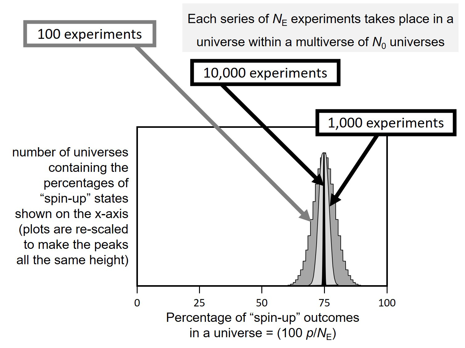
experiments is ( ) E E 0 3 1 number of universes with outcomes 4 4 p N p N p N p − ↑ = ↑ ↓ (8) In Figure 3 we show equation (8) plotted as histograms for the outcomes of three different series of 60º experiments, containing, in each universe, _N_E = 100, 1,000 and 10,000 experiments respectively. We have rescaled each of these three histograms so that their peaks are all the same height.
In the series of 10,000 experiments per universe, we see that in virtually all of the _N_0 universes, the number of spin-up outcomes in a universe is almost exactly ¾ of the total number of experiments in that universe (that is, in this case, 7,500). Taking the width of the peak to be proportional to the percentage standard deviation of the plot, namely,
| 100 N E | 3 1 × 4 4 |
|---|
, it will be seen that, as the number of experiments in the series, _N_E, increases, so the percentage of spin-up outcomes more closely matches the ideal result of 75% predicted by the Born rule for a series containing an indefinitely large number of 60º experiments in virtually every one of the parallel universes in which the series takes place. This echoes Saunders’ observation (Saunders [31]) that “branches recording relative frequencies of outcomes of repeated measurements at variance with the Born rule have, collectively, much smaller amplitude than those that do not (vanishingly small, given sufficiently many trials)”.
In summary, following Everett’s thought experiment, we have shown that, if the numbers of universes with given outcomes are apportioned across the MDW multiverse according to the Born rule for those outcomes as in expression (6), then, in a series of experiments within any single one of these universes, the results will generally be consistent with Born rule predictions.
For clarity, we repeat the assertion in the first paragraph of Section: The Frequency Distribution of Universes in MDW we have not attempted to derive the Born rule in any way— we have assumed the Born rule, and then we have shown that experiments in any given universe to demonstrate the Born rule will be successful if the numbers of universes in the multiverse are distributed according to the Born outcome probabilities for those experiments.
Entanglement in MDW
Suppose that two particles are emitted in opposite directions along the y-axis in an entangled singlet state where the total spin is zero, and that the spin of each particle is measured with a Stern-Gerlach detector set at an angle θ to the other, as measured in the x-z plane. In MDW, we consider the two separate measurements of two entangled particles as a single event. Pictorially, in any given universe, the two measurements are embedded at two different spacetime locations, and may be spacelike separated. The probability amplitudes for all four possible (mutually exclusive) outcomes may be written
1 sin 2 2 θ ↑↑; 1 cos 2 2
θ ↑↓; 1 cos 2 2
θ ↓↑ and
1 sin 2 2 θ ↓↓.
where the first arrow always represents the spin of the first particle and mutatis mutandis for the second arrow.
Hence, the absolute square of the probability amplitude for a match, (m), where( ) (
$$ (m) = \left(\left| \uparrow \uparrow \right\rangle o r \left| \downarrow \downarrow \right\rangle\right), \mathrm {i s} $$ $$ \left(\frac {1}{2} \sin^ {2} \frac {\theta}{2} \uparrow \uparrow + \frac {1}{2} \sin^ {2} \frac {\theta}{2} \downarrow \downarrow\right) = \sin^ {2} \frac {\theta}{2} (m). $$ .
Similarly, the absolute square of the probability amplitude for a non-match, (n), where ( ) (
$$ (n) = \left(\left| \uparrow \downarrow \right\rangle o r \left| \downarrow \uparrow \right\rangle\right), $$ is ( ) 2 cos 2 n θ . Here, the brackets around “m” and “n” mean that the terms are used purely indicatively and have no numerical value in this position.
If we put θ = 120º, the probabilities for a match and a non-match are, respectively, ¾ and ¼. Therefore, in a series of _N_E entanglement experiments, from expression (6), the number of universes containing $m$ matched and $(N_E - m)$ non-matched outcomes in any particular order of outcomes
is $N_0 \left( \frac{3}{4}(m) \right)^m \left( \frac{1}{4}(n) \right)^{(N_E - m)}$, so that, taking account of all possible combinations, the total number of universes in which there are $m$ matches and $(N_E - m)$ non-matches in a series of $N_E$ entanglement experiments is
$$\text{number of universes with } m \text{ matched outcomes} = N_0 \left( \frac{N_0}{m} \right) \left( \frac{3}{4}(m) \right)^m \left( \frac{1}{4}(n) \right)^{(N_E - m)}.$$
Since this is in the same form as equation (8), then the results of series of entanglement experiments can be represented by Figure 3 where we substitute "matching" for "spin-up" in the text for the two axes. So we come to the equivalent conclusion, that, if we continue to repeat the above entanglement experiment a sufficiently large number of times in any single, given universe, then it is increasingly likely that we shall be able to demonstrate that we are in a universe where the proportion of matching outcomes approaches the result of $\frac{3}{4}$ predicted by quantum mechanics for this entanglement experiment.
In treating the two measurements of the entangled particles as a single event, we are recognizing that the outcomes are distributed across the multiverse just as described in Section: The Frequency Distribution of Universes in MDW, so that, in any given universe (our own, for instance), the detection of one of the pair has no effect on the detection of the other. This echoes the comment of Boughn [49]:
"[...] the magic of the correlations of Bell’s entangled system is a direct consequence of the quantum behavior of a single spin $\frac{1}{2}$ particle."
Spatiotemporally Finite Universes in a Finite Multiverse
We used angles of $60^\circ$ and $120^\circ$ to illustrate the above thought experiments because the outcome probabilities are rational. This means that the number of identical universes with a given configuration can be integer, from expression (6). However, probabilities predicted by quantum mechanics are generally irrational. This raises the question of whether or not the multiverse is finite with regard to the number of universes in it. If it is not uncountably infinite, then quantum mechanics will turn out to be only an ideal approximation (no matter how accurate) to the actual structure of the multiverse according to MDW.
To answer the question of finitude, consider, for the moment, weighted universes as in Figure 2(b) rather than the multiple universes of Figure 2(c), and recall that our use of the term "universe" refers to its complete spatiotemporal extent after decoherence. Suppose that such a weighted universe contains $m$ mutually independent quantum events: for example, $m$ non-entangled events, each of which is located at a spacelike distance from all the others. Since each of these events must have at least two possible outcomes, then there are at least $2^m$ possible combinations of outcomes, with at least $2^m$ configurations of weighted universes containing these outcomes.
Recalling from Section: Beyond the Cosmological Particle Horizon that events in a universe are not limited to the finite volume within the particle horizon, we begin by supposing that $m$ is countably infinite, which would mean an uncountable infinity (at least $2^m$) of weighted universes in the multiverse.
In any universe, if we trace the cause of any event successively backwards in time, we shall ultimately arrive at the same root event that is common to all universes. In the multiverse of our supposed uncountable infinity of universes, the number of universes containing an outcome of an event directly caused by the root event must also be uncountably infinite. In turn, the number of universes containing a succeeding outcome will also be uncountably infinite. Proceeding thus, we see that every outcome of every event in such an uncountably infinite multiverse will be contained in an uncountably infinite number of universes.
In such a multiverse, the intuition is that it is not meaningful to speak of the probability of being in a universe with any particular configuration of outcomes. If so, then demonstrating the Born rule by conducting a series of $60^\circ$ experiments within a given universe would not work, because it would no longer be meaningful to say that in nearly every universe the percentage of spin-up outcomes matches the 75% predicted by the Born rule within a specified limit. Nevertheless, if we regard each weighted universe with a given percentage of spin-up outcomes as the sole element of a set, then might the problem be amenable to a measure such as the Lebesgue measure?
Measure-Theoretic Discussion
The Lebesgue measure is a standard mathematical tool for dealing with infinite sets. It can be used, for instance, if we can arrange for the elements of the sets that we are interested in to be strung out along the number line (or it could be an area rather than the number line, or a volume, or an even higher-dimensional space). As an example, the probability of randomly picking a specific real number between zero and one is literally zero, because the number of real numbers is uncountably infinite. Given that, one might conclude that that the probability of randomly picking a real number with a value between, say, 0.4 and 0.5 cannot be calculated. However, intuitively, the chance must be one in ten: see Figure 4(a). It is this intuition that is formalized by the mathematics of the Lebesgue measure.
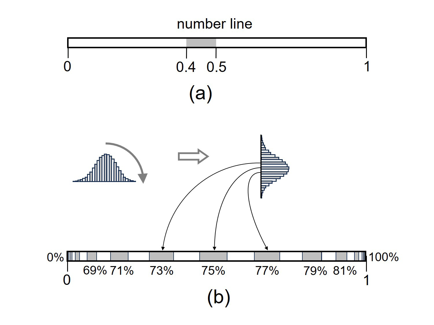
If each one of the uncountably infinite number of universes in the multiverse contained only the outcomes of the series of 60º experiments, then the Lebesgue measure might indeed be used. Recalling Figure 3 to show this heuristically, the histogram bars for the series of, for instance, 100 experiments could be laid end-to-end, as it were, on the interval [0, 1] of the number line, and the probability of being in a universe with, say, 71 spin-up outcomes would simply be the interval on [0, 1] corresponding to the length of the 71% histogram bar (see Figure 4(b)).
Why the Lebesgue Measure Fails in this Instance
However, in our proposed scenario, there is a countably infinite number of other events, m, which also have to be included in the configuration of each weighted universe in addition to the 60º experiments, and it is these events that ultimately preclude the use of the Lebesgue measure. To see why, first imagine a universe containing no events except for a single 60º experiment. Then there is one weighted universe for each of the two possible outcomes of the experiment. Let us regard these two universes as two distinct sets, each containing just one element: the first set contains an element which is a universe with a spin-up outcome and the second set contains an element which is a universe with a spin-down outcome. If there were just one other independent event in each of these two universes, say event B1, with outcomes of, say, spin-up and spin-down, then the original set with the universe containing a 60º result of spin-up would have to be divided into two non-intersecting sets: one set containing a universe—again, a single element—where the 60º result is spin-up and the outcome of B1 is also spin-up, and the other set containing a universe—again, a single element— where the 60º result is still spin-up but the outcome of B1 is spin-down. These two sets are non-intersecting because the single element contained in the first set is different from the single element contained in the second. The set where the 60º result is spin-down would similarly be split into two non-intersecting sets by the same event B1, giving a total of four non-intersecting sets.
If we include another independent event, B2, then this divides each of the four sets again, and so it will become clear that, with a countably infinite number, m, of independent events in each universe where a single 60º experiment is performed, the total number of non-intersecting sets, 2_m_+1, is uncountably infinite. If we now consider not just one, but many 60º experiments in a series, as in Figure 3, in an attempt to demonstrate the Born rule, the result is the same—we end up with an uncountably infinite number of pairwise disjoint (i.e., all non-intersecting) sets.
And this is why the Lebesgue measure fails: the measures of an uncountably infinite number of sets would have to be added together, but then the Lebesgue measure requires that the pairwise disjoint sets forming the sum must be countably additive—it will not handle uncountable additivity (see, for instance, Richardson ([50], pp: 8)). A union of an uncountably infinite number of pairwise disjoint sets of universes would require uncountable additivity, which will give inconsistent results (for a more detailed discussion, see, for instance, Miller ([51], pp: 65-70)). So, despite the original hope of using the Lebesgue measure, it turns out that, in this case, the original intuition was correct: experiments to demonstrate the Born rule will at best return inconsistent results.
In summary, if the universes in the multiverse contain just a countably infinite number of events, so that the number of universes in the multiverse is uncountably infinite, then, in any such universe, any series of experiments to measure quantum probabilities will return results which are inconsistent with the Born predictions. Clearly, this is also the case for events numbered in higher cardinalities. Since we do not live in such an inconsistent universe, the conclusion is (1) that there is not an uncountably infinite number of universes in the multiverse; and so (2) they do not contain even just countably infinite numbers of events (because that would lead to an uncountably infinite multiverse): the number of quantum events in any universe must be finite.
The argument at the beginning of this section started with weighted universes. The conclusion of a finite multiverse of finite universes is unchanged if we transform from weighted universes to multiple identical copies of universes in proportion to the weightings, in accordance with the MDW structure as in Figure 2(c).
Recalling the observation at the beginning of this section about irrational quantum probabilities, note that the finitude of the multiverse implies that the number of alternative basis states for any outcome is never infinite. That implies that, for instance, it must take only a finite number of possible positions to account for all possible interactions registering on the detecting screen of a two-slit experiment. This approximation to the quantum ideal of an infinitely finely grained screen should not be seen as a fundamental impediment, because, in practice, the constituent atoms of the screen will determine the basis, limiting it to a finite number of distinct detecting locations.
The consequences of a finite number of quantum events in any universe are significant. The cosmological principle of isotropy and homogeneity extends beyond our own particle horizon, and so, if our universe were spatially infinite, then the number of events would also be infinite. Given the finite number of events in our complete spacetime, we conclude that our isotropic and homogeneous universe must be spatially finite. (Notice that a finite number of events in our complete spacetime implies that our future is also finite, inasmuch as there must be one final event in the far distant future, which is indeed conceivable. So, in that sense, we can say that our universe is also temporally finite.) Astronomical observations that we are living in a spatially flat universe (e.g. Aiola, et al. [52], Aghanim, et al. [53]) do not necessarily negate our conclusion that our universe is spatially finite, because the observed flatness can be explained by models of inflation (e.g. Starobinskii [54], Guth [55], Linde [56]). As it happens, inflation does not necessarily rule out using the universe’s topology as a means of falsifying our finite-universe conjecture. Since the topology of the universe will still be the same now as it was initially, current work (e.g., Asselmeyer-Maluga, et al. [57], Thébault [58]) may lead to future developments in cosmology that will suggest ways to determine the topology of the pre-inflationary universe, which would then be a test of its spatial finiteness, and therefore of MDW.
Discussion
The MDW picture of discrete universes diverging from each other rather than branching at every interaction is essentially that of modal realism described by Lewis [32]. However, the motivation for our proposal stems ultimately from the need to account for quantum uncertainty, whereas Lewis developed his thesis from a different philosophical perspective, lying outside of the ambit of this paper. The case for discrete, diverging universes is also considered by Saunders and Wallace [33], Saunders [4], Wallace [21], Wilson [34]. None of these authors, though, promotes the notion of a finite number of discrete, diverging universes, with Wallace saying that you shouldn’t think of each universe as an individual unit (his picture is of “slabs” of universes) and Wilson being agnostic on whether the number of universes is either finite or infinite. Deutsch [59] argues for a continuous infinity of worlds. No author uses their model to deduce that the universes in MWI are spatially finite.
Authors who consider an uncountable infinity (a continuum) of universes include Deutsch [60], Boström [61], Holland [62], Poirier [63], Parlant, et al. [64], Schiff and Poirier [65]. (Others, such as Wilson ([34], pp: 178) accept the possibility of a continuum of universes, but are open to the prospect that the number may yet be finite.) Exceptionally, Hall, et al [29], Vaidman [42] and Sebens [66], among a few others, are unconvinced by the notion of a continuum of universes, the latter two authors making the case that regions containing infinite densities of worlds cannot be compared in assessing probabilities of being in a particular world.
Returning for a moment to the two papers of Hall, et al [29] and Sebens [66], their authors having arrived independently at essentially the same quantum interpretation, the key idea is to apply the quantum potential of the de Broglie-Bohm interpretation not just to particles in a single universe but to particles in a configuration space containing a finite number of discrete universes. However, in contrast to the universes in MDW, these universes appear effectively to interact, ultimately as a result of how the de Broglie-Bohm quantum potential determines the configurations of universes in this interpretation. This interaction is most clearly manifest as a mutual repulsion in configuration space, which increases with increasing similarity between the worlds. This would effectively rule out universes being identical, or indeed identical for any significant part of their trajectories, whereas such identical universes are integral to the MDW interpretation.
Boström [61] maintains that it is legitimate to use the Lebesgue measure over a continuum of universes, effectively pointing out that, with universes that are continuous in configuration space, the Lebesgue measure can be used as a measure of the proportions of universes contiguously adjacent to each other sharing a particular state. However, while his argument would be correct for universes containing, for instance, only a series of 60º experiments, that contiguity is broken by the uncountable number of unrelated outcomes, which is another way to view the above argument that the Lebesgue measure cannot cope with an uncountably infinite number of pairwise disjoint sets of universes.
MDW shares some features of the many-threads picture described by Barrett [67]. Each thread is the history—the “experience”—of one trajectory through the dendritic tracery of MWI. In contrast to MDW, however, where two or more identical universes are allowed, there is apparently only one thread for each trajectory upwards through the branches, and there is an infinite number of threads in its multiverse.
Identification of Discrete Worlds
In Section: The Frequency Distribution of Universes in MDW, we assigned a unique identifier—a label, i, —to each universe, even when these universes were otherwise identical. Here is the reason for these identifiers. For the Born rule to work through self-locating uncertainty, there must always be collections of universes which are identical to each other after decoherence (for illustration, see Figure 2(c)). This has a consequence if we take the view of those authors such as, for instance, Tegmark [68] or McKenzie [69], who consider our universe as purely a mathematical structure. The problem is that any given mathematical structure is unique—there cannot be another separate, yet identical, mathematical structure, any more than there can be a separate mathematical structure which is identical to an existing structure such as, say, the set of the first ten prime numbers. It would be like asking whether we can have another integer that is identical to 4.
The resolution is that these identical universes must in fact be part of a larger, integrated mathematical structure, namely the multiverse. By “integrated”, we mean that, from the perspective of the multiverse, individual universes must be indexed or labelled so that they are identified as distinguishable substructures of the multiverse. In this way, from the internal perspective of any universe, it is one of many identical universes, giving rise to the uncertainty of the outcome of a quantum interaction, while, from the external perspective of the multiverse, these substructures are not identical, because they can be distinguished as different, indexed parts of the overarching mathematical structure of the multiverse. Hence, the problem of having identical mathematical structures doesn’t arise.
Conclusion
We have presented the case for a fixed, finite number of discrete, non-splitting, non-interacting, spatiotemporally finite, decohered spacetimes emerging from Everett’s Universal Wave Function. The MDW approach gets round the problem of why an observer should give more credence to being in universes with greater branch weights by using the “branch counting” method. This divides universes with given branch weights into multiple identical universes in numbers proportional to the branch weights. As expected, probabilities derived from branch weights according to Gell Mann and Hartle [24] are equal to those calculated for the corresponding discrete universes in the MDW picture.
We showed that each universe should be considered as containing all decohered outcomes over the entire extents of their spacetimes, including events/interactions occurring beyond any cosmological particle horizon. We also showed that a series of experiments as prescribed by Everett within a universe will demonstrate consistency with the Born rule. It turns out that a countably infinite number of interactions needs an uncountably infinite number of universes, and we showed why measures such as the Lebesgue measure would fail in that case, with the result that the Born rule would not be demonstrable. This leads us to conclude that the number of universes in the multiverse must be finite and, as a corollary, that the universes are finite in space and duration.
In summary, the scope of Many Discrete Worlds is the same as that of the Many Worlds Interpretation, with Everett’s Universal Wave Function evolving according to Schrödinger’s equation, accounting for indeterminism (through self-locating uncertainty), while the branch-weight problem of MWI is avoided (because in MDW all universes are equally weighted). In addition, if the assumption is made that the multiverse and its component universes are essentially mathematical structures, then identical universes are nevertheless distinguishable as distinct substructures of the multiverse.
While one or more of the above features of MDW are to be found in other interpretations of quantum mechanics, the force of the arguments in this paper strongly suggests to us that, uniquely, these features are combined in our multiverse of Many Discrete Worlds.
References
-
Freire O, Bacciagaluppi G, Darrigol O, Hartz T, Joas C, et al. (Eds.) (2022) The Oxford Handbook of the History of Quantum Interpretations. Oxford University Press.
-
Everett H III (1957) Relative state formulation of quantum mechanics. Rev Mod Phys 29: 454-462.
-
Saunders S, Barrett J, Kent A, Wallace D (2010) Many worlds? Everett, quantum theory, and reality. Oxford University Press, Oxford.
-
Saunders S (2010) Many Worlds? An introduction. In: Saunders, et al. (Eds.), Many worlds? Everett, quantum theory, and reality. Oxford University Press.
-
Kent A (1990) Against Many-Worlds interpretations. Int J Mod Phys A 5(9): 1745-1762.
-
Kent A (2010) One world versus many: The inadequacy of Everettian accounts of evolution, probability, and scientific confirmation. In: Saunders S, et al. (Eds.), Many Worlds? Everett, Quantum Theory, and Reality. Oxford University Press.
-
Butterfield J (1996) Whither the minds? Br J Philos Sci 47(2): 200-221.
-
Butterfield J (2001) Some worlds of quantum theory. In: Russell RJ, et al. (Eds.), Quantum mechanics: Scientific perspectives on divine action. Vatican Observatory Publications, pp: 111-140.
-
Hartle JB (2010) Quasi classical realms. In: Saunders S, et al. (Eds.), Many Worlds? Everett, Quantum Theory, and Reality. Oxford University Press.
-
Greaves H, Myrvold W (2010) Everett and evidence. In: Saunders S, et al. (Eds.), Many Worlds? Everett, Quantum Theory, and Reality. Oxford University Press.
-
Zurek WH (2010) Quantum jumps, Born’s rule, and objective reality. In: Saunders S, et al. (Eds.), Many Worlds? Everett, Quantum Theory, and Reality. Oxford University Press.
-
Barrett J (2011) Everett’s pure wave mechanics and the notion of worlds. Eur J Philos Sci 1: 277-302.
-
Tappenden P (2011) Evidence and uncertainty in Everett’s multiverse. Br J Philos Sci 62: 99-123.
-
Tappenden P (2019) Everett’s multiverse and the world as wavefunction. Quantum Rep. 1: 119-129.
-
Tappenden P (2023) Set theory and many worlds. Quantum Rep 5(1): 237-252.
-
Adlam E (2014) The problem of confirmation in the Everett interpretation. Stud Hist Philos Sci B Stud Hist Philos Mod Phys 47: 21-32.
-
Papineau D, Rowe T (2023) The MWI and Distributive Justice. Quantum Rep 5: 224-227.
-
Vaidman L (2023) Special Issue: The Many-Worlds Interpretation of Quantum Mechanics. Quantum Reports, MDPI.
-
Belnap N (1992) Branching space-time. Synthese 92: 385-434.
-
Bacciagaluppi G (2002) Remarks on Space-Time and Locality in Everett’s Interpretation. In: Placek T, et al. (Eds.), Non-locality and Modality. Springer, Dordrecht.
-
Wallace D (2012) The Emergent Multiverse: Quantum Theory According to the Everett Interpretation. Oxford University Press, Oxford.
-
Marvian I, Lidar DA (2015) Quantum speed limits for leakage and decoherence. Phys Rev Lett 115: 210402.
-
Hartle JB (1993) The quantum mechanics of closed systems. In: Hu BL, et al. (Eds.), Directions in Relativity. Cambridge University Press.
-
Gell-Mann M, Hartle JB (2007) Quasiclassical coarse graining and thermodynamic entropy. Phys Rev A 76: 022104.
-
Boughn S (2018) Making sense of the Many Worlds Interpretation, Arxiv 1801: 08587.
-
DeWitt BS (1970) Quantum mechanics and reality. Phys Today 23(9): 30-35.
-
Vaidman L (1998) On schizophrenic experiences of the neutron or why we should believe in the Many-Worlds Interpretation of quantum theory. International Studies in the Philosophy of Science 12: 245-261.
-
Wilson A (2013) Objective probability in Everettian quantum mechanics. Br J Philos Sci 64(4): 709-737.
-
Hall MJW, Deckert DA, Wiseman HM (2014) Quantum phenomena modeled by interactions between many classical worlds. Phys Rev X 4: 041013.
-
Werner F (1962) Transcript of Conference on the Foundations of Quantum Mechanics, Xavier University Cincinnati (1 October 1962), with Everett’s remarks.
-
Saunders S (2010) Chance in the Everett interpretation. In: Saunders S, et al. (Eds.), Many worlds? Everett, quantum theory, and reality. Oxford University Press.
-
Lewis DK (1986) On the Plurality of Worlds. Blackwell.
-
Saunders S, Wallace D (2008) Branching and uncertainty. Br J Philos Sci 59: 293-305.
-
Wilson A (2020) The Nature of Contingency: Quantum Physics as Modal Realism. Oxford University Press.
-
Khawaja J (2025) Conquering Mount Everett: Branch counting versus the Born Rule. Br J Philos Sci 77(2).
-
Saunders S (2021) Branch-counting in the Everett interpretation of quantum mechanics. Proc R Soc A 477(2255): 20210600.
-
Barrett J, Goldbring I (2024) Everettian Mechanics with Hyperfinitely Many Worlds. Erkenntnis 89: 1367-1386.
-
Short AJ (2023) Probability in many-worlds theories. Quantum 7: 971.
-
Davis TM, Lineweaver CH (2004) Expanding Confusion: Common Misconceptions of Cosmological Horizons and the Superluminal Expansion of the Universe. Publ Astron Soc Aust 21(1): 97-109.
-
Saunders S (1998) Time, quantum mechanics, and probability. Synthese 114: 373-404.
-
Vaidman L (2012) Probability in the Many-Worlds Interpretation of quantum mechanics. In: Ben-Menahem Y, et al. (Eds.) Probability in Physics. Springer-Verlag, pp: 299.
-
Vaidman L (2014) Quantum theory and determinism. Quantum Stud Math Found 1: 5-38.
-
Sebens CT, Carroll SM (2018) Self-locating uncertainty and the origin of probability in Everettian quantum mechanics. The British Journal for the Philosophy of Science 69(1): 25-74.
-
McQueen KJ, Vaidman L (2019) In defence of the self- location uncertainty account of probability in the many- worlds interpretation. Stud Hist Philos Sci B Stud Hist Philos Mod Phys 66: 14-23.
-
Dawid R, Friederich S (2022) Epistemic separability and Everettian branches—A Critique of Sebens and Carroll. Br J Philos Sci 73(3): 711-721.
-
Deutsch D (1999) Quantum theory of probability and decisions. Proc R Soc Lond A 455: 3129-3137.
-
Wallace D (2010) How to prove the Born rule. In: Saunders S, et al. (Eds.), Many Worlds? Everett, Quantum Theory, and Reality. Oxford University Press.
-
Barnum H, Caves CM, Finkelstein J, Fuchs CA, Schack R (2000) Quantum Probability from Decision Theory? Proc R Soc Lond A 456: 1175-1182.
-
Boughn S (2017) Making sense of Bell’s theorem and quantum nonlocality. Found Phys 47: 640-657.
-
Richardson LF (2009) Measure and Integration. John Wiley and Sons.
-
Miller SJ (2017) The Probability Lifesaver: All the Tools You Need to Understand Chance. Princeton University Press.
-
Aiola S, Calabrese E, Maurin L, Naess S, Schmitt BL, et al. (2020) The Atacama Cosmology Telescope: DR4 maps and cosmological parameters. J Cosmol Astropart Phys (12): 47.
-
Aghanim N, Akrami Y, Ashdown M, Aumont J, Baccigalupi C, et al. (2020) Planck 2018 results. Astron Astrophys 641.
-
Starobinskii AA (1979) Spectrum of relict gravitational radiation and the early state of the universe. Soviet Journal of Experimental and Theoretical Physics Letters 30: 682-685.
-
Guth AH (1981) Inflationary universe: a possible solution to the horizon and flatness problems. Phys Rev D 23: 347-356.
-
Linde AD (1982) A new inflationary universe scenario: A possible solution of the horizon, flatness, homogeneity, isotropy and primordial monopole problems. Phys Lett B 108(6): 389-393.
-
Asselmeyer-Maluga T, Król J, Wilms A (2022) Big Bang and topology. Symmetry 14(9): 1887.
-
Thébault KPY (2023) Big bang singularity resolution in quantum cosmology. Class Quantum Grav 40: 055007.
-
Deutsch D (1985) Quantum Theory as a Universal Physical Theory. Int J Theor Phys 24(1): 1-41.
-
Deutsch D (1997) The Fabric of Reality. Penguin Press.
-
Boström KJ (2015) Quantum mechanics as a deterministic theory of a continuum of worlds. Quantum Stud Math Found 2: 315-347.
-
Holland P (2005) Computing the wavefunction from trajectories: Particle and wave pictures in quantum mechanics and their relation. Ann Phys 315(2): 505-531.
-
Poirier B (2010) Bohmian mechanics without pilot waves. Chem Phys 370: 4-14.
-
Parlant G, Ou YC, Park K, Poirier B (2012) Classical- like trajectory simulations for accurate computation of quantum reactive scattering probabilities. Comput Theor Chem 990: 3-17.
-
Schiff J, Poirier B (2012) Communication: Quantum mechanics without wavefunctions. J Chem Phys 136(3): 031102.
-
Sebens CT (2015) Quantum mechanics as classical physics. Philos Sci 82: 266-291.
-
Barrett J (1999) The quantum mechanics of minds and worlds. Oxford University Press, Oxford.
-
Tegmark M (2008) The Mathematical Universe. Found Phys 38(2): 101-150.
-
McKenzie A (2020) Reality and Super-Reality: Properties of a Mathematical Multiverse. Axiomathes 30: 453-478.
- The Genesis of Psychopathology
- Noentarion: Toward a New Ontological Category for Non Biological Agency in the Postmodern Age
- The Place of Wittgenstein’s Tractatus in the History of Philosophy
- Digital Hermeneutics Embodied in Brian Kim Stefans’ “The Dreamlife of Letters,” and Memory: Analog to Flash Interface in the Light of Ecofeminism
- Using C-Tables to Teach Class Logic
- The Ideology of Education’s Postponed Fantasies: Deepenings on a Pressing Problematic