Macroscale Habitat Assessment and Suitability Modeling of Riverine-Segregated Eco-Geographic Units of Church’s Sideband (Monadenia churchi), within and surrounding the Greater Trinity Basin, Northern California, USA
Church’s Sideband (Monadenia churchi) is a medium-sized endemic terrestrial snail with a broad geographic distribution. It provides an excellent opportunity to evaluate habitat variance across a diverse geologic, topographic, and ecologic landscape. Herein I document and model variance in macrohabitat characteristics of five riverine-segregated Eco-geographic Units (populations) within the range of the species (Mad and Sacramento rivers, and Northern, South-Central, and Western basins). The most common forest cover-types were Sierra Mixed Conifer (49.6%), Douglas Fir (14.1%), and Montane Hardwoodconifer (8.7%). Statistical comparisons showed significant differences in 93.3% of the cover-types among groups. Principal Components Analysis of macroscale biotic and abiotic ecological variables accounted for 51.7% of the combined variance along both vectors for the species. K-means clustering using Multidimensional Scaling showed good separation of point-samples for the Sacramento River and Western Basin, but there was considerable overlap in point-samples among the remaining groups. All Habitat Suitability Models showed suitable habitat widely distributed throughout the range of M. churchi, but most areas consisted of Low suitability interspersed with few areas of Moderate to High “quality” habitat. For all groups, Generalized Additive Model regression of grid-cell density against macroclimatic co-variates exhibited the best fit compared to models of Forest Structure and Exposure-Distance to Nearest Stream. Dot-plots of variable importance, produced by Random Forest Regression, showed that predictor categories with importance values > 10 were: 1) Macroscale Climate (64.0%, n = 78), followed by Exposure-Distance to Nearest Stream (20.0%), and Forest Stand Structure (16.0%).
Introduction
Delineation of suitable habitat is vital to the success or failure of species management, particularly as relates to the potential release or relocation of focal special status taxa. A primary objective in site selection is finding areas with the most desired ecological conditions. This process is generally based on a priori defined qualitive or quantified species-specific habitat criteria. Initially, most criteria used in evaluating species-driven site selection for management purposes are of a geographic nature. This means that site selection is a spatially driven process. Also, evaluation of landscape-level variance in preferred ecological affinities generally requires a multi-criteria decision-making process, which results in development habitat suitability models (HSM) based on species-driven site preferences. Identification of multiple macroscale site-specific attributes, by use of synergistic modeling of environmental criteria, may also contribute to the efficiency, quantity, and quality of spatial analyses used for potential site selection in areas previously not surveyed. Information on the geographic distributions, spatial relationships, and habitat affinities of terrestrial gastropod communities in northern California is largely nonexistent [1, 2]. Habitat criteria for most taxa have been poorly documented, rarely quantified, and based largely on anecdotal natural history information obtained during proximate-level species inventories [3, 4, 5, 6, 7]. Knowledge of the geographic scope and macroscale ecological detail of suitable habitat of terrestrial mollusks is, therefore, critical to the understanding of the habitat requirements of a particular taxon for the purpose of resource conservation, especially at the community level.
For example, Church’s Sideband (Klamath) land snail (Monadenia churchi) is a medium-sized endemic terrestrial mollusk found in several northern California counties (Figure 1) [8]. This taxon is considered reflective of a species that occurs at many locations over a large geographic range. The historical and current distribution of M. churchi, and other terrestrial snails, in this region represents relics of the Late (Upper) Pleistocene Epoch (~129,000 and c. 11,700 years ago), when climate was much cooler and more mesic than today [9]. Historically, populations of M. churchi were referenced in the context of “western” and “eastern” segments with only anecdotal information on plant community type found throughout a diverse and complex topographic landscape. It was hypothesized that habitat associations varied between these segments. At the time, it was though that eastern populations tended to inhabit mostly rocky riparian corridors, whereas western populations tended to dwell within more upland sites of late-serial forest, mixed- conifer forest, pine-oak woodlands, or within riparian vegetation composed of various rock types [10, 11].
Without reference to eastern or western segments, a predictive habitat model found that on average M. churchi occurred most frequently in areas dominated by late-seral hardwood (oak = Quercus spp.) cover and basal area, which lacked late successional forest characteristics at either a macro- or micro-habitat scale [1]. Yet quantification of suitable habitat at either scale is lacking for this taxon. Importantly, there has been no documented assessment (ecologically or genetically) of the potential significance of geographic or topographic discontinuities, including potential stream valleys or more importantly the major riverine barriers that encompass the full geographic range of M. churchi.
As such, M. church provides an excellent opportunity to evaluate macroscale environmental variance across a diverse geographic, topographic, and ecological landscape. My specific research objectives were fivefold. First, I evaluated and quantified variance in biotic and abiotic environmental attributes at a macroscale using Geographic Information Systems (GIS) data layers. This allowed me to describe differences variation among point samples for the M. churchi and for each riverine-segregated cluster of point-samples (Eco-geographic Unit [EGU]; [12]). Second, I developed HSMs models based on species-driven site-specific preferences. Binary (presence-absence) data were not used in my analyses. Third, I developed hypothesized estimates of grid-cell density generated from habitat preferences obtained from the original point-sample occurrence data. Fourth, I used regression models to fit and compare hypothesized density estimates (response variable) to individual and categories of environmental predictors (explanatory variables or drivers) for the species and each of the five EGU within M. churchi. My study provides baseline documentation for spatial decision support and habitat suitability useful in applied management of M. churchi, which was aimed at facilitating future conservation planning and potential listing status.
Methods and Materials
Study Area
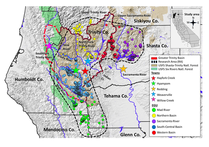
My research focused on the range of M. church within a segment of the Klamath Bioregion centered on the Greater Trinity Basin, northern California. This area includes Humboldt, Mendocino, Shasta, Siskiyou, Tehama, and Trinity counties, and much of the Shasta-Trinity and Six Rivers National forests (Figure 1). Importantly, this area is bisected by several major river systems. Within this zone there is abundant Douglas fir (Pseudotsuga menziesii), white fir (Abies concolor), ponderosa pine (Pinus ponderosa), sugar pine (P. lambertiana), incense cedar (Calocedrus decurrens), tanoak (Notholithocarpus densiflorus), and Pacific madrone (Arbutus menziesii) forest cover-types. At its southwest boundary, this segment of the basin also intergrades with montane coastal forest of the North Coast Bioregion [13]. Watersheds within the basin are mostly within mountainous terrain, with the only level land in a few narrow valleys (Weaverville Basin, and Hyampom and Hayfork valleys) dominated by mixed conifer and hardwood forest, narrow riparian corridors of white alder (Alnus rhombifolia), big leaf maple (Acer macrophyllum), and various species of willow (Salix spp.).
Basin uplands consist of deciduous hardwood understories of Pacific madrone, giant chinquapin (Castanopsis chrysophylla), tanoak, and canyon live oak (Quercus chrysolepis) cover- types as far south as Mendocino County. Foothills of the western slope of the Sacramento River Valley (Shasta and Tehama counties) sport major forest cover and vegetation- types, which proceed downslope through Klamath mixed conifer forest, patches of montane hardwoods, progressively tapering riparian corridors, montane and mixed assemblages of chaparral, and annual grassland [14]. Climate of the region tends to be Mediterranean, with cool, wet winters and hot, dry summers. Average annual precipitation over the Trinity River watershed is ~1400 mm. Precipitation ranges from ~940 mm in lowlands to as high as ~2200 mm [15]. Approaching the northern Sacramento River Valley average annual temperatures range from ~27.8℃ in July to ~7.8℃ in December. The wettest month is December (~90.7 mm rain), and average annual precipitation is ~429.3 cm/yr.
Eco-geographic Units (EGU)
Point-samples of M. churchi were a priori grouped into five EGUs: 1) Mad River, 2) Northern Basin, 3) Sacramento River, 4) South-Central Basin, and 5) Western Basin (Figure 1). Each EGU was delineated based on the presence of historically defined large-scale riverine systems (natural breaks), which encompassed the full geographic range of the species within and adjacent to the Greater Trinity Basin. Placement of EGUs was not based on GIS watershed delineations. Watershed data layers tend to be mostly arbitrarily that describe the physics of water movement in a defined space [16]. They and are not generally intended as a management tool for biological use, assessing genetic relatedness, or evaluating patterns of historical biogeography among biological or ecological units (S. dymond, University of California, Davis; pers. comm. 2015). This is because watershed data layers are not always indicative of connected or disconnected hydrological systems. For example, within the geographic range of M. churchi several watersheds transcend opposite sides of the Trinity, South Fork Trinity, Mad, and Sacramento rivers. Further, some tributary creeks (Italian, Swede) are in the same watershed, but they are not connected hydrologically [2].
Data Collection and Survey Methods
I obtained Universal Transverse Mercator (UTM) survey coordinates for point-samples (occurrence points) of M. churchi during surveys of M. setosa for genetic analyses [17]. Field surveys focused on historical qualitative accounts of suitable habitat for M. churchi based on documented searches [18, 19]. I sampled active snails during warm, wet, foggy, or rainy conditions during March to May and September
to October 2008 and 2009. I focused on areas by use of opportunistic visual search based on historical descriptions of suitable microhabitat, which was rapid (~30 min/per site) and entailed neither degradation nor soil removal [20, 21]. I also used geo-rectified point-samples from inventory plots developed by the Department of Agriculture, United States Forest Service, Six Rivers National Forest obtained from the Northwest Forest Plan’s Survey and Manage program [10, 22]. Point-samples collected by USFS were conducted weduring the spring by use of a stratified random procedure [4, 5] when daytime temperature was > 5C° and soil was moist as determined by touch. Each plot was sampled for terrestrial mollusks twice, with a minimum of 10-days between surveys. Searches targeted the most likely mollusk habitat by inspecting “preferred” features (downed wood, rocks, ferns) within a 5-m radius surrounding that feature (ecological stratification [23]). In total, I included 2949 M. churchi point-samples. I used GIS-based Landsat Visual Ecological Groupings (CALVEG; [24]) and California Wildlife Habitat Relationships (CWHR; [25, 26, 27]) to assess geographic variation in point-samples for forest cover-type vegetation and forest stand structure. CWHR is a habitat classification information system and predictive CWHR forest stand cover-types Attributes AGS = Annual grassland, BAR = Barren, BOP = Blue oak-foothill pine, CPC = Closed-cone pine cypress, DFR = Douglas fir, KMC = Klamath mixed conifer, LAC = Lacustrine, MCH = Mixed chaparral, MCP = Montane chaparral, MHC = Montane hardwood conifer, MHW = Montane hardwood , PPN = Ponderosa pine, SCN = Subalpine conifer, SMC = Sierran mixed conifer, WFR = White fir. GIS datasets were captured at 1:1,000,000 scale; minimum mapping size of ~2.5-hectar pixels.
model for terrestrial wildlife, It is based on the assumption that wildlife species respond to forest structure within a ~16.2-ha minimum mapping unit. A minimum mapping size of ~2.5-ha pixels was used to contrast CWHR in forest cover- type attributes for each point-sample.
I used 15 environmental predictor variables to evaluate macroscale habitat preferences (Table 1). From these I created four sets of covariant categories describing macroscale environmental variance: 1) Forest Cover-type (CALVEG), 2) Forest Stand Structure (CWHR), 3) Macroscale Climate measures obtained from geo-rectified raster data for Northern California [28, 29], and 4) properties of the landscape describing exposure and distance from a point- sample to the nearest stream (henceforth referred to as Exposure-Distance to Stream), which were generated from 10-m digital elevation models. Because Forest Cover-type is purely a descriptive variable, I only used covariants in categories 2, 3, and 4 to model habitat suitability and to assess estimates of grid-cell density in M. churchi and each EGU separately.
Forest Stand Attributes (Conifer Cover from above [CCFA], Hardwood cover from above [HCFA], Over-story Tree Diameter [OSTD], Total Tree cover from above [TCFA], Tree Size Class[TSIZ]) CALVEG vegetation cover from above (mapped vegetation [%] cover [crown] from above) by aerial photos. Total tree cover, Conifer tree cover, and Hardwood cover from above mapped as a function of canopy closure in 10% cover classes: 0 (< 1%), 5 (1 – 9%), 15 (10 – 19%), 25 (20 – 29%), 35 (30 – 39%), 45 (40 – 49%), 55 (50 – 59%), 65 (60 – 69%), 75 (70 – 79%), 85 (80 – 89%), and 95 (90 – 100%). CALVEG overstory tree diameter class mapped mixed tree types using average diameter at breast height (DBH = 1.37 m above ground) for trees forming the uppermost canopy layer [30] using average basal area (Quadratic Average Diameter or QMD; [31]) of top tree story categories: 1 = seedlings (0 – 2.3 cm QMD), 2 = saplings (2.5 – 12.5 cm QMD), 3 = poles (12.7 – 25.2 cm QMD), 4 = medium sized trees (50.8 – 76.0 cm QMD), and 5 = large sized trees (> 76.2 cm QMD). Tree size classification derived from mapped attributes corresponding to parameters derived from the CALVEG and CWHR systems. Tree size codes (ranked): 1 = seedling tree, 2 = sapling tree, 3 = pole tree, 4 = small tree, 5 = medium-large tree, and 6 = multilayered tree. Map product a scale of 1:24,000 to 1:100,000. 1:100,000.
Average Monthly Macroscale Climate Attributes (Summer Temperature [TASM ℃], Winter Temperature [TAWN ℃], Summer Precipitation [PASM mm], Winter Precipitation [PAWN mm]) Average monthly climate attributes were derived from the PRISM (2024; [29, 32]) where long-term average datasets were modeled using a spatially gridded digital elevation model (DEM) as the predictor grid for specific climatological periods. Values were based on monthly 30-yr average “normal” datasets covering the conterminous US, averaged over the period 1991-2020 and included both “historical” and current climate trends. Monthly data were scaled at 2.5 (4 km) resolution.
Covariant predictor category (Aspect [ASPC], Elevation [ELEV m], Hill-shade [HLSD], Slope[SLOP], Distance to Nearest Stream [DNST m]) Maps of aspect, elevation, hill-shade, and slope were all derived from a United States Geological Survey (USGS) Digital Elevation Model (DEM; 1:250,000-scale/3-arc second resampled to 10-m resolution). Aspect obtained from a raster surface that identified down-slope direction of maximum rate of change in value from each cell to its neighbors. Equates to slope direction and values of each cell in the output raster show compass direction of surfaces measured clockwise in degrees from zero (due north) to 360° [33]. Degree’s aspect in direction = north = 0°, east = 90°, south = 180°, and west = 270°. Values of cells in an aspect dataset indicate direction cell’s slope faces. Flat areas of no down slope direction = value of -1. Aspect quantified by use of aspect degrees binned into one of eight 45° ordinal categories (N, NE, E, SE). Elevation (m) obtained from vertical units of a spaced grid with values referenced horizontally to UTM projections referenced to North American Datum NAD 83. Hill-shade was obtained from a shaded relief raster (integer values ranging from 0 – 255). The output raster only considered local illumination angle. Analysis of shadows considered effects of local horizon at each cell. Shadowed raster cells received a value of zero. Slope was obtained from a raster surface that identified gradient or rate of maximum change in z-value from each cell of a raster surface. It relates maximum change in elevation over distance between a cell and its eight neighbors, thus identifying the steepest downhill descent from the cell [33]). Range of slope values (0° - 360°; flat = 0°, steep = 35° to 45°, moderate = 5° to 8.5°, and very steep > 45°). Distance to the nearest stream obtained from CDFW GIS Clearing house (CDFWGIS 2024). Although this measurement is generally related to more proximate (microhabitat) conditions, these primary order streams/rivers may potentially reflect mesic/riparian conditions within the watershed at a macroscale-level.
Statistical Analyses
I performed all analyses using programs that run on the R Statistical Software platform (ver.4.3.3) and set statistical significance at α < 0.05. I evaluated univariate normality in habitat parameters using the adjusted Anderson-Darling test (AD; Package “nortest” v1.0-4). All tests for normality failed (Figure 2). Thus, I used nonparametric statistics to evaluate significance in follow-on tests of environmental variance. I evaluated fit distributions by visual use of density histograms, and several theoretical density distributions using the Package “fitdistrplus” (v1.1-11, functions “fitdist”, “gofstat”, “AIC”). I determined the best fit distribution to the data by use of Akaike’s goodness of fit criterion (AIC). The smaller the AIC the better the fit.
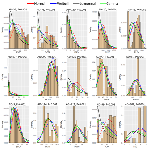
Figure 2: Histograms of theoretical density distributions for environmental parameters measured for each point-sample throughout the range of the M. churchi. ASPC = Aspect, CCFA = Conifer Cover from Above, D.Est. = Estimated Grid-cell Density, DNST = Distance to Nearest Stream (m), ELEV = Elevation, HCFA = Hardwood Cover from Above, HLSD = Hill-shade, OSTD = Over-story Tree Diameter, PASM = Average Annual Summer Precipitation (mm), PAWN = Average Annual Winter Precipitation (mm), SLOP = Slope, TASM = Average Annual Summer Temperature (℃), TAWN = Average Annual Winter Temperature (℃), TCFA = Total Tree Cover from Above, and TSIZ = Tree Size Class; AD = Anderson-Darling statistics.
I used Kruskal-Wallis non-parametric ANOVA rank sum test (X_2; Package “stats” v3.62) to evaluate the null hypothesis of no overall significant difference between _M. churchi and among EGUs for each environmental variable, and in Random Forest Regression [34, 35]. When the omnibus test was rejected in variable relationships post-hoc pairwise comparisons were made using the Dunn test statistic (Z). I adjusted p-values using the Bonferroni correction method (α = 0.99) to counteract the problem of inflated Type I errors when engaging in multiple pairwise comparisons. I used non-parametric Spearman’s rank correlation 2-tailed test (rs; Package “easystats” v0.7.1) to calculate the strength and direction of the relationship between pairs of variables whether linear or not.
To avoid variables becoming dominant due to different or large measure units, I scaled all the data to unite variance (mean = 0, and standard deviation = 1) when running Principal Components Analysis (Program “FactoMineR”). I used this unconstrained method of ordination to identify the extent of association, assess the relative ability of each parameter to explain variation among EGUs, and explore variance in macrohabitat data decomposed into PC axes (vector) when plotted along the first two axes. I used classical nonlinear Metric Multidimensional scaling, in combination with K-means clustering, as a visual representation of the distance (similarities) relationships among EUG’s point- data based all environmental data (MDS; Package “stats” v3.62). MDS is a flexible and adaptable technique that: 1) can handle complex data, 2) is not restricted to linear projections of the data (it is nonlinear), 3) can be applied to a wide range of information, including numerical, categorical, and mixed data, and allows exploration of relationships in lower-dimensional space (2D) for easier interpretation [35, 36]. I used K-means clustering to visualize structure among river-segregated EGUs relative to the 2D-dimensional relationships displayed in the PCA for the species. A K-means iterative algorithm was used to partitioned EGUs into pre- defined non-overlapping EGU (cluster), where each point- sample belongs to only one EGU. It makes the intra-cluster point-data as similar as possible while keeping clusters as different (far) as possible. Point-data were assigned to a cluster such that the sum of the squared distance between point-data and the cluster’s centroid (arithmetic mean of all point-data within that cluster) was at the minimum.
Because my data were not normally distributed, I used Generalized Additive Modeling (GAM; Package “mgcv” v1.8- 34; [37]) in all regressions of D.Est. (response variable) with environmental predictors. This method: 1) is a semi- parametric extension of Generalized Linear Models (GLM), which extends multiple linear regression to allow for non- linear relationships between response and explanatory variables; and 2) is flexible enough to handle complex patterns;
and 3) it can capture intricate, non-linear relationships that traditional linear models cannot represent [38, 39]. Because my data were positive real valued and predominately right- skewed (Figure 2). I used a Gamma error-structure for the non-exponential GAM family distribution to establish the relationship between continuous non-negative response variable(s) and the smoothed functions of predictor variables [40]. Statistics reported from each GAM regression included parametric coefficients for the intercept (mean of predicted/ response values [y]) and various other standard statistics (estimate, standard error, t-value, P-value). Other statistics included: 1) Ref.df = degrees of freedom used to compute test statistics, 2) GAM F statistic = approximate significance of the smooth terms, 3) R2(adj) = proportion of variance in the response variable explained by predictor variables by adjusting for the number of predictors in the model, 4) Dev.Exp. = the proportion of null deviance explained most appropriate for non-normal errors, 5) p-value and 95% confidence bands for spline lines, and 6) effective degrees of freedom (edf). The edf values estimated from GAM models were used as a proxy to evaluate the degree of non-linearity in driver-response relationships. In all GAMs I used the “gam. check” function (replications [rep] = 500) to evaluate model diagnostics. Models with the low AIC values was deemed “best-fit.”
Habitat Suitability Model
I attached GIS raster and vector data layers of environmental variables to all snail observed point- samples. I then generated a set of 100000 (100k) random- points contained within an arbitrary “Research Area” (RA) surrounding the known geographic range of M. churchi (Figure 1). The boundary of the RA extended ~3 km in all directions beyond any known historical sample point for M. churchi. I chose a ~3 km boundary around the RA to potentially include any unsampled areas adjacent to known samples, given the species’ limited movement, niche tolerances, and abiotic and biotic interactions [41]. From the original point-samples I computed standard statistics for all variables by species and for each EGU separately. I computed minimum values for each variable. I then added each value, one-by-one in a string of minimums, for use as selection criteria to query the 100k random-points for the species and each EGU separately (Table 2). This approach provided a simple method of selecting variables from all attributes for use in generating hypothesized suitability maps from throughout the range of M. churchi and for each EGU, and in areas where sampling has historically not occurred. The resulting HSMs were displayed by us of kernel density heatmaps for each group separately. Polygonising each raster heatmap quantified the approximate hectares in each suitability category (Low, Moderate, and High), based on natural breaks in abundance of kernel densities for each group.
Evaluation of the performance of HSMs is generally accomplished by testing a model against population measures, such as species density or reproductive success [42, 43, 44, 45]. The assumption being that the relationship between the response variable and a selected environmental predictor (or suite of predictors) signals high “quality” species-specific habitat conditions [46]. Previous studies have demonstrated that for macroscale climate models, areas of good habitat correlate significantly with areas of high abundance, while the reverse is also true [47, 48]. Thus, to obtain comparative estimates of hypothesized point-sample densities associated with macroscale measures of environmental attributes I: 1) generated a 500 x 500 m grid-cell polygon layer within the boundaries of the RA, 2) overlayed the 100k random- points onto the grid, and 3) attached random-points that fell within each grid-cell to its respective centroid. This process produced 993 estimates of D.Est across the species range and within the boundaries of each EGU. I assumed that hypothesized areas with high D.Est values were indicative of high-quality habitat. I also assumed that each environmental predictor functioned in a single driver-response relationship for the covariants within the three predictor categories (Forest Stand Structure, Macroscale Climate, Exposure- Distance to Stream). A check on sampling error for point- samples throughout the range of M. churchi found no significant correlation between D.Est. and distance to the nearest road from where snails were observed (rs = -0.050, p = 0.119, n = 993 grid-cell). This indicated that there was no bias in sampling in relation to proximity to road access.
| M. churchi (n = 2949) | Mad River (n = 297) | ||||||||||
|---|---|---|---|---|---|---|---|---|---|---|---|
| Variable | x | Min | Max | Range | SD | vars | x | Min | Max | Range | SD |
| ASPC | 163.6 | 1 | 360 | 359 | 102.5 | ASPC | 172.4 | 1 | 358 | 357 | 99.1 |
| CCFA | 43.9 | 1 | 95 | 94 | 26.1 | CCFA | 49 | 1 | 95 | 94 | 24.5 |
| D.Est | 6.2 | 1 | 27 | 26 | 5.3 | D.Est. | 5.2 | 1 | 15 | 14 | 4.1 |
| DIST | 468.3 | 0.3 | 1774.2 | 1773.9 | 308.1 | DIST | 540.7 | 18.5 | 1774.2 | 1755.7 | 321.8 |
| ELEV | 987.7 | 324 | 1822 | 1498 | 389.6 | ELEV | 1135.4 | 725 | 1741 | 1016 | 177.5 |
| HCFA | 11.8 | 1 | 95 | 94 | 19.1 | HCFA | 17 | 1 | 95 | 94 | 20.8 |
| HLSD | 210.2 | 116 | 255 | 139 | 29.1 | HLSD | 210 | 116 | 255 | 139 | 34 |
| OSTD | 19 | 1 | 40 | 39 | 10.1 | OSTD | 22.2 | 1 | 40 | 39 | 9.9 |
| PASM | 40.5 | 22.8 | 72.9 | 50.1 | 11 | PASM | 41.3 | 22.8 | 55.8 | 33 | 7.6 |
| PAWN | 1243.6 | 637.9 | 1837 | 1199.1 | 259.7 | PAWN | 1173.4 | 719.5 | 1485.1 | 765.6 | 128.4 |
| SLOP | 32.4 | 1 | 88 | 87 | 15.2 | SLOP | 32.1 | 1 | 88 | 87 | 14.6 |
| TASM | 21.1 | 15.2 | 25.6 | 10.4 | 2.5 | TASM | 19.7 | 16.4 | 22.2 | 5.8 | 1.2 |
| TAWN | 5.9 | 0.8 | 9.7 | 8.9 | 2 | TAWN | 5.2 | 2.5 | 7.1 | 4.6 | 0.8 |
| TCFA | 56.2 | 1 | 95 | 94 | 28.5 | TCFA | 66.9 | 1 | 95 | 94 | 23.4 |
| TSIZ | 3.9 | 1 | 5 | 4 | 1.3 | TSIZ | 4.3 | 1 | 5 | 4 | 1.1 |
| Northern Basin (n = 125) | Sacramento River (n = 722) | ||||||||||
| vars | x | Min | Max | Range | SD | vars | x | Min | Max | Range | SD |
| ASPC | 181.9 | 1 | 359 | 358 | 99 | ASPC | 162.6 | 1 | 360 | 359 | 108.2 |
| CCFA | 55 | 1 | 95 | 94 | 26.1 | CCFA | 24.7 | 1 | 85 | 84 | 25.6 |
| D.Est | 3.1 | 1 | 9 | 8 | 2.3 | D.Est. | 9.9 | 1 | 27 | 26 | 7.2 |
| DIST | 447.9 | 15.5 | 1724.7 | 1709.2 | 390.7 | DIST | 340.2 | 0.3 | 1151.8 | 1151.5 | 262.3 |
| ELEV | 959.2 | 340 | 1822 | 1482 | 276.4 | ELEV | 420.2 | 324 | 1117 | 793 | 118.7 |
| HCFA | 6.1 | 1 | 85 | 84 | 13.7 | HCFA | 24.4 | 1 | 95 | 94 | 25.1 |
| HLSD | 212.5 | 122 | 255 | 133 | 30.3 | HLSD | 215.5 | 141 | 255 | 114 | 24.9 |
| OSTD | 22.5 | 1 | 40 | 39 | 9 | OSTD | 14.6 | 1 | 40 | 39 | 11.5 |
| PASM | 35.9 | 28 | 59 | 31 | 7.3 | PASM | 44.4 | 37.8 | 72.9 | 35.1 | 6.4 |
| PAWN | 826.3 | 637.9 | 1334.3 | 696.4 | 79.5 | PAWN | 1343.8 | 1219.6 | 1837 | 617.4 | 83.8 |
| SLOP | 32.7 | 1 | 86 | 85 | 16.9 | SLOP | 30.6 | 1 | 78 | 77 | 15.8 |
| TASM | 19.9 | 15.2 | 21.9 | 6.7 | 1.1 | TASM | 24.9 | 19.4 | 25.6 | 6.2 | 0.7 |
| TAWN | 4.3 | 0.8 | 6.6 | 5.8 | 0.9 | TAWN | 9.1 | 4.5 | 9.7 | 5.2 | 0.6 |
| TCFA | 60.9 | 1 | 95 | 94 | 25.6 | TCFA | 50.5 | 1 | 95 | 94 | 38 |
| TSIZ | 4.3 | 1 | 5 | 4 | 1.2 | TSIZ | 3.2 | 1 | 5 | 4 | 1.6 |
| South-Central Basin (n = 1294) | Western Basin (n = 511) | ||||||||||
| vars | x | Min | Max | Range | SD | vars | x | Min | Max | Range | SD |
| ASPC | 163.2 | 1 | 360 | 359 | 100.5 | ASPC | 156.4 | 1 | 357 | 356 | 101.5 |
| CCFA | 50.3 | 1 | 95 | 94 | 21.1 | CCFA | 49.5 | 1 | 85 | 84 | 25.9 |
| D.Est | 4.3 | 1 | 16 | 15 | 3.4 | D.Est. | 7 | 1 | 16 | 15 | 4.1 |
| DIST | 465.1 | 1.1 | 1427.3 | 1426.2 | 285.3 | DIST | 620.4 | 3.6 | 1441.9 | 1438.3 | 313.3 |
| ELEV | 1201 | 325 | 1789 | 1464 | 253.4 | ELEV | 1171 | 345 | 1601 | 1256 | 199.6 |
| HCFA | 5.7 | 1 | 85 | 84 | 11.5 | HCFA | 7.9 | 1 | 85 | 84 | 15.2 |
| HLSD | 209.5 | 131 | 255 | 124 | 28 | HLSD | 204.2 | 127 | 255 | 128 | 32.3 |
| OSTD | 20.1 | 1 | 40 | 39 | 8.3 | OSTD | 20 | 1 | 40 | 39 | 10.7 |
| PASM | 32 | 24.4 | 52.9 | 28.5 | 4.3 | PASM | 57.4 | 27 | 67.5 | 40.5 | 7.5 |
| PAWN | 1134.6 | 741.9 | 1671.1 | 929.2 | 262.9 | PAWN | 1521.6 | 710.9 | 1742.4 | 1031.5 | 162.2 |
| SLOP | 31.3 | 2 | 87 | 85 | 14.3 | SLOP | 38 | 4 | 74 | 70 | 15 |
| TASM | 19.2 | 17.8 | 21.9 | 4.1 | 0.8 | TASM | 21.7 | 17.1 | 25.6 | 8.5 | 1.3 |
| TAWN | 4.7 | 3.9 | 6.6 | 2.7 | 0.6 | TAWN | 5.4 | 2.7 | 9.4 | 6.7 | 0.9 |
| TCFA | 56 | 1 | 95 | 94 | 22.7 | TCFA | 57.4 | 1 | 95 | 94 | 27.4 |
| TSIZ | 4.1 | 1 | 5 | 4 | 1 | TSIZ | 4 | 1 | 5 | 4 | 1.4 |
Table 1: Standard statistics for the species and each EGU point-sample of _M. churchi_. SD = Standard Deviation. *Forest Stand St
Table 2: Standard statistics for the species and each EGU point-sample of M. churchi. SD = Standard Deviation. *Forest Stand Structure (CCFA = Conifer Cover from Above, HCFA = Hardwood Cover from Above, OSTD = Over-story Tree Diameter, TCFA = Total Tree Cover from Above, and TSIZ = Tree Size Class). *Mesoscale Climate (PASM = Average Annual Summer Precipitation, PAWN = Average Annual Winter Precipitation, TASM = Average Annual Summer Temperature, TAWN = Average Annual Winter Temperature. *Exposure-Distance (ASPC = Aspect, DNST = Distance to Nearest Stream (m), ELEV = Elevation, HLSD = Hill-shade, SLOP = Slope. Hypothesized cell density = D.Est. and x̅ = average for each value.
Random Forest Regression
I used the Package “randomForest” (v4.7-1.1; [34, 35, 48, 49]) to check the “importance” of individual predictor variables on determining D.Est. This algorithm was executed as a regression for each group. I modeled 2001 trees using 75% of the D.Est. and the remaining 25% as independent test data. The Random Forest model used five variables at each split. The method uses the percent increase in the mean squared error (%IncMSE) of predictions (estimated with out-of-bag-CV) as a result of variable j being permuted (values randomly shuffled; [50, 51]). It is the average difference between the predicted value for D.Est. and the observed value. The higher the value of %IncMSE the more important the variable is to the regression model.
A negative number signals that the random variable worked better and was not predictive enough to be important.
In the Random Forest analyses, I used two different metrics to measure the quality of the HSM. First, I used the Mean Absolute Error (MAE), which measures the average absolute difference between the true value of an observation and the value predicted by the model; low values for MAE indicate a better model fit. Viewed in combination, these metrics provided an idea of how well the model might perform on previously unseen data. Second, I used %VExp., which is the proportion of the variance in the response variable explained by predictor variables. The higher the %VExp the better the driver variables can predict the response variable, and the stronger the correlation between response and predictor.
Results
Current Geographic Range of the Species
I estimated the geographic range of M. churchi to be ~11800 km2 based on the total area encompassed by all documented point-samples. Importantly, I view all estimates of the area occupied by M. churchi to be conservative pending more extensive sampling in all cardinal directions. The greatest geographic separation among EGUs occurs along a rather well-defined west-to-east longitudinal gradient and a more well-defined north-to-south latitudinal gradient (Figure 1). Topographically, separation among EGUs occurs along both north and south sides of the mainstem Trinity River in Trinity and Siskiyou counties. To the west EGUs were separated between the Trinity River and both the western and eastern sides of the upper Sacramento River and expansive Sacramento Valley (Shasta Co.). In the mid-portion of the Greater Trinity Basin EGUs were separated between both mainstems of the Trinity River and the South Fork Trinity River (Trinity Co.). To the south EGUs were separated by the mainstem South Fork Trinity River and the west-to-east orientation of the South Fork Mountain range adjacent to the Mad River watershed (Trinity and Mendocino Cos.), and the western edge of the Sacramento River and Sacramento Valley (Tehama Co.). Small tributaries flow into the Trinity River (North Fork Trinity River, New River, Canyon Creek) on the northern side of the mainstem. Whereas the South Fork Trinity River receives the Hayfork Creek tributary at its head along the eastern slope of South Fork Mountain adjacent to the Trinity-Humboldt County Divide [17].
Differences in Forest Cover-Type Attributes
I identified 15 CWHR macroscale forest cover-types when all point-samples for the species were combined (Figure 3). The most common cover-type was Sierra Mixed Conifer Forest (SMC = 49.6%), followed by Douglas Fir Forest (DFR = 14.1%), and Montane Hardwood-conifer (MHC = 8.7%). Among EGUs the most common forest cover-type was: 1) Sierra Mixed Conifer Forest (SMC) for all groups except the Sacramento River EGU; 2) Douglas Fir Forest (DFR; Mad River, Northern Basin, and South-Central Basin); and 3) Montane Chaparral (MCP; Western Basin). The Sacramento River EGU exhibited the greatest overall diversity in the number of forest-cover types.
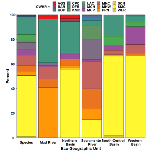
Figure 3: Bar graphs of percent frequency of forest stand cover-types for the M. churchi and each Eco-Geographic Unit (EGU). Wildlife Habitat Relationships (CWHR) forest stand cover-types are: AGS = Annual grassland, BAR = Barren, BOP = Blue oak-foothill pine, CPC = Closed-cone pine cypress, DFR = Douglas fir, KMC = Klamath mixed conifer, LAC = Lacustrine, MCH=Mixed chaparral, MCP = Montane chaparral, MHC = Montane hardwood conifer, MHW = Montane hardwood, PPN = Ponderosa pine, SCN = Subalpine conifer, SMC = Sierran mixed conifer, and WFR = White fir.
Evaluation of the total percentage of all CWHR forest cover-types revealed that all pair-wise comparisons between M. churchi and among EGUs were significantly correlated (Table 3). M. churchi exhibited the strong correlations with all EGUs except the Northern Basin. However, not all EGUs were significantly correlated with each other. Similarities in cover- type was strongest between the Mad River and Northern basin EGUs, and the Sacramento River and the Western Basin EGUs. While the South-Central Basin was most strongly correlated with the Western Basin and Mad River.
| Taxon/EGU | Species | Mad River | Northern Basin | Sacramento River | South-Central Basin | Western Basin |
|---|---|---|---|---|---|---|
| M. churchi (n = 2949) | ------- | 0.001*** | 0.045* | 0.002** | 0.007** | 0.001*** |
| Mad River (n = 297) | 0.79 | ------- | 0.001*** | 0.014** | 0.184 | 0.009** |
| Northern Basin (n = 125) | 0.52 | 0.81 | ------- | 0.139 | 0.387 | 0.045* |
| Sacramento River (n = 722) | 0.74 | 0.62 | 0.40 | ------- | 0.688 | 0.12 |
| South-Central Basin (n = 1294) | 0.66 | 0.36 | 0.24 | 0.11 | ------- | 0.003** |
| Western Basin (n = 511) | 0.78 | 0.65 | 0.52 | 0.42 | 0.71 | ------- |
Table 2: Spearman rank (rs) correlations of percentage groups based on CWHR 15 macroscale CWHR cover-types obtained at point-samp
Correlation among Environmental Variables
For the species, all environmental attributes except Hill-shade, Slope, and Total Cover from Above were significantly correlated with UTM-East; and all attributes except Aspect, Distance to Nearest Stream, Hill-shade, over story Tree Diameter, and Tree Size were significantly correlated with UTM-N (p-values < 0.05) (Table 4). However, the strength of these relationships varied considerably. For all environmental variables, the highest positive correlations with both UTM coordinate vectors were with Average Monthly Summer and Winter Precipitation and Temperature. Among environmental variables the highest positive correlations were between Average Monthly Summer and Winter Temperatures, and Overstory Tree Diameter and Tree Size. The highest negative correlations were between Elevation and Average Monthly Summer and Winter Temperatures, respectively.
| Variable | UTM-E | UTM-N | ASPC | CCFA | D.Est. | DIST | ELEV | HCFA | HLSD | OSTD | PASM | PAWN | SLOP | TASM | TAWN | TCFA | TSIZ |
|---|---|---|---|---|---|---|---|---|---|---|---|---|---|---|---|---|---|
| UTM-E | -------- | 0.00*** | 0.01** | 0.00*** | 0.00*** | 0.00*** | 0.00*** | 0.00*** | 0.59 | 0.00*** | 0.00*** | 0.00*** | 0.09 | 0.00*** | 0.00*** | 0.84 | 0.00*** |
| UTM-N | 0.56 | -------- | 0.21 | 0.00*** | 0.00*** | 0.33 | 0.00*** | 0.00*** | 0.15 | 0.39 | 0.00*** | 0.00*** | 0.00*** | 0.00*** | 0.00*** | 0.00*** | 0.28 |
| ASPC | -0.05 | -0.02 | -------- | 0.00*** | 0.45 | 0.59 | 0.05* | 0.30 | 0.00*** | 0.00*** | 0.18 | 0.03* | 0.00*** | 0.00*** | 0.00*** | 0.00*** | 0.00*** |
| CCFA | -0.32 | -0.09 | 0.09 | -------- | 0.00*** | 0.69 | 0.00*** | 0.00*** | 0.00*** | 0.00*** | 0.00*** | 0.38 | 0.00*** | 0.00*** | 0.00*** | 0.00*** | 0.00*** |
| D.Est | 0.34 | 0.23 | -0.01 | -0.19 | -------- | 0.11 | 0.00*** | 0.00*** | 0.95 | 0.00*** | 0.00*** | 0.00*** | 0.85 | 0.00*** | 0.00*** | 0.03* | 0.00*** |
| DIST | -0.08 | -0.02 | 0.01 | -0.01 | -0.03 | -------- | 0.00*** | 0.80 | 0.17 | 0.27 | 0.00*** | 0.00*** | 0.74 | 0.00*** | 0.00*** | 0.16 | 0.90 |
| ELEV | -0.49 | -0.33 | 0.04 | 0.31 | -0.33 | 0.30 | -------- | 0.80 | 0.17 | 0.27 | 0.00*** | 0.00*** | 0.74 | 0.00*** | 0.00*** | 0.16 | 0.90 |
| HCFA | 0.29 | 0.13 | 0.02 | -0.31 | 0.15 | 0.00 | -0.39 | -------- | 0.37 | 0.00*** | 0.00*** | 0.00*** | 0.36 | 0.00*** | 0.00*** | 0.00*** | 0.00*** |
| HLSD | 0.01 | -0.03 | 0.41 | 0.14 | 0.00 | 0.03 | -0.02 | -0.10 | -------- | 0.00*** | 0.40 | 1.00 | 0.00*** | 0.3 | 0.70 | 0.02* | 0.00*** |
| OSTD | -0.14 | -0.02 | 0.14 | 0.59 | -0.10 | -0.02 | 0.13 | 0.12 | 0.07 | -------- | 0.23 | 0.07 | 0.00*** | 0.00*** | 0.00*** | 0.00*** | 0.00*** |
| PASM | 0.66 | 0.55 | -0.02 | -0.12 | 0.28 | 0.09 | -0.15 | 0.18 | -0.02 | -0.02 | -------- | 0.00*** | 0.00*** | 0.00*** | 0.00*** | 0.00*** | 0.68 |
| PAWN | 0.31 | 0.30 | -0.04 | 0.02 | 0.08 | 0.13 | 0.17 | -0.05 | 0.00 | -0.03 | 0.64 | -------- | 0.17 | 0.00*** | 0.02* | 0.84 | 0.13 |
| SLOP | 0.03 | 0.17 | 0.06 | 0.12 | 0 | -0.01 | -0.02 | 0.17 | -0.29 | 0.10 | 0.09 | 0.03 | -------- | 0.00*** | 0.00*** | 0.00*** | 0.00*** |
| TASM | 0.75 | 0.62 | -0.06 | -0.36 | 0.39 | -0.09 | -0.74 | 0.38 | -0.02 | -0.2 | 0.51 | 0.09 | 0.1 | -------- | 0.00*** | 0.17 | 0.00*** |
| TAWN | 0.59 | 0.38 | -0.06 | -0.41 | 0.35 | -0.09 | -0.75 | 0.42 | -0.01 | -0.26 | 0.35 | 0.04 | 0.06 | 0.90 | -------- | 0.65 | 0.00*** |
| TCFA | 0 | 0.07 | 0.08 | 0.60 | -0.04 | -0.03 | -0.09 | 0.53 | 0.04 | 0.59 | 0.08 | 0 | 0.25 | 0.03 | 0.01 | -------- | 0.00*** |
| TSIZ | -0.14 | -0.02 | 0.15 | 0.62 | -0.1 | 0 | 0.15 | 0.09 | 0.07 | 0.84 | -0.01 | -0.03 | 0.12 | -0.2 | -0.27 | 0.59 | -------- |
Table 3: Pair-wise Spearman rank correlations (rs) between macroscale GIS-based environmental attributes measures at point- sampl
Table 4: Pair-wise Spearman rank correlations (rs) between macroscale GIS-based environmental attributes measures at point- samples where M. churchi were observed. Correlation coefficients are below the diagonal and probabilities are above. *Forest Stand Structure (CCFA = Conifer Cover from Above, HCFA = Hardwood Cover from Above, OSTD = Over-story Tree Diameter, TCFA = Total Tree Cover from Above, and TSIZ = Tree Size Class). *Mesoscale Climate (PASM = Average Annual Summer Precipitation, PAWN = Average Annual Winter Precipitation, TASM = Average Annual Summer Temperature, TAWN = Average Annual Winter Temperature. * Exposure-Distance (ASPC = Aspect, DNST = Distance to Stream, ELEV = Elevation, HLSD = Hill-shade, SLOP = Slope); UTM-E = UTM East and UTM-N = UTM North. The correlation between summer and winter temperatures was high but they were kept as data because they represent seasonal trends. Variables with the strongest pairwise correlations (> 50%) are bolded; p-values: 0.05 = *, 0.01 = *, 0.001 = *.
Forest Structure, Climate, and Exposure- Distance to Stream Attributes
Principal Components Analysis of habitat parameters for M. churchi accounted for only 51.7% of the total dispersion (variance) among attributes on the first two components. Vector loadings, direction, and the relationship of each attribute arrow showed that Elevation and all forest stand elements had the highest positive loadings along PC I (27.0%) (Figure 4). Conversely, environmental attributes summarizing monthly Average Annual Summer and Winter Temperatures, and Precipitation loaded negatively along this vector, whereas Slope, Hill-shade, and Distance to Stream plotted at or near the origin. Along PC II (24.7%) all variables plotted positive except Elevation and Distance to Nearest Stream.
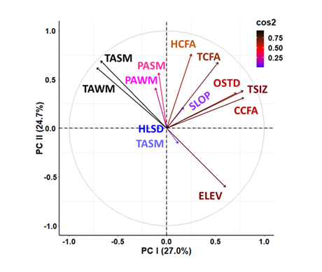
Figure 4: Principal Components Analysis (PCA) of macroscale environmental variable measured at each point-sample where M. churchi was found. Categories and predictors are: 1) Forest Stand Structure (CCFA = Conifer Cover from Above, HCFA = Hardwood Cover from Above, OSTD = Over-story Tree Diameter, TCFA = Total Tree Cover from Above, and TSIZ = Tree Size Class); 2) Mesoscale Climate (PASM = Average Annual Summer Precipitation, PAWN = Average Annual Winter Precipitation, TASM = Average Annual Summer Temperature, TAWN = Average Annual Winter Temperature; 3) Exposure-Distance (DNST = Distance to Nearest Stream (m), ELEV = Elevation, HLSD = Hill-shade, SLOP = Slope. Aspect was left out of the analysis because there were no significant differences among EGUs. The cos2 color index positions variables based on their contribution and quality of representation along each vector (blue color = low, black color = high).
K-means clustering of macroscale environmental variables showed good separation along both MDS I and MDS II for point-samples from the Sacramento River and Western Basin EGUs (95% confidence ellipses), but there was considerable overlap among point-samples for the remaining EGUs (Figure 5). The Western Basin averaged the highest levels of precipitation, mostly in the form of rain (Table 2). While point-samples along PC I within the Sacramento River EGU were a function of being found predominantly within down-slope foothill and lower valley habitats, characteristic of the more arid upper Sacramento Valley. These regions were significantly lower in elevation, had less extensive conifer cover from above, and higher levels of seasonal monthly average temperatures, compared to more montane forest environs. Point-samples within the South- Central Basin EGU were the most expansive ecologically and occupied an intermediate position between and within the Northern Basin and the Mad River EGUs. Non-parametric ANOVA showed significant overall differences among groups for all environmental variables (Table 5). Ensuing post-hoc pairwise comparisons showed significant differences for all environmental variables except aspect for all groups. This variable was removed from further analyses.
| Mad-Eel River | Northern Basin | Sacramento River | South-Central Basin | ||||||||
|---|---|---|---|---|---|---|---|---|---|---|---|
| Conifer Cover from Above (CCFA): x 2 = 150.5, p < 0.001***; 70% significant | |||||||||||
| EGU | Z | p-adj | Z | p-adj | Z | p-adj | Z | p-adj | |||
| NB | 3.5 | 0.003** | |||||||||
| SR | 7.5 | 0.001*** | SR | 9.2 | 0.001*** | ||||||
| SC | 1.8 | 0.400 | SC | 5.1 | 0.001*** | SC | 8.3 | 0.001*** | |||
| WB | 1.7 | 0.500 | WB | 2.5 | 0.065 | WB | 11 | 0.001*** | WB | 4.5 | 0.001*** |
| x 2 Hardwood Cover from Above (HCFA): = 72.0, p < 0.001***; 40% significant | |||||||||||
| EGU | Z | p-adj | Z | p-adj | Z | p-adj | Z | p-adj | |||
| NB | 1 | 1 | |||||||||
| SR | 3.1 | 0.013** | SR | 2.4 | 0.095 | ||||||
| SC | 3.6 | 0.002** | SC | 0.6 | 1.000 | SC | 8.2 | 0.001*** | |||
| WB | 1.5 | 0.667 | WB | 1.8 | 0.359 | WB | 0.9 | 1.000 | WB | 4.8 | 0.001*** |
| Overstory Tree Diameter (OSTD): x 2 = 51.3, p < 0.001***; 70% significant | |||||||||||
| EGU | Z | p-adj | Z | p-adj | Z | p-adj | Z | p-adj | |||
| NB | 2.2 | 0.134 | |||||||||
| SR | 3.9 | 0.001*** | SR | 5.2 | 0.001*** | ||||||
| SC | 4 | 0.001*** | SC | 5.2 | 0.001*** | SC | 0.5 | 1.000 | |||
| WB | 0.9 | 1.000 | WB | 3 | 0.015* | WB | 3.5 | 0.002** | WB | 3.7 | 0.001*** |
| Total Cover from Above (TCFA): x 2 = 205.5, p < 0.001***; 60% significant | |||||||||||
| EGU | Z | p-adj | Z | p-adj | Z | p-adj | Z | p-adj | |||
| NB | 1.7 | 0.447 | |||||||||
| SR | 0.2 | 1.000 | SR | 2 | 0.249 | ||||||
| SC | 9.5 | 0.001*** | SC | 4.5 | 0.001*** | SC | 12 | 0.001*** | |||
| WB | 4.3 | 0.001*** | WB | 1.3 | 0.988 | WB | 5.3 | 0.001*** | WB | 5.6 | 0.001*** |
| Tree Size Class (TSIZ): x 2 = 114.4, p < 0.001***; 80% significant | |||||||||||
| EGU | Z | p-adj | Z | p-adj | Z | p-adj | Z | p-adj | |||
| NB | 2.3 | 0.117 | |||||||||
| SR | 6.9 | 0.001*** | SR | 7.4 | 0.001*** | ||||||
| SC | 5.3 | 0.001*** | SC | 6.1 | 0.001*** | SC | 3.2 | 0.008** | |||
| WB | 0.6 | 1.000 | WB | 2.8 | 0.025* | WB | 7.4 | 0.001*** | WB | 5.7 | 0.001*** |
| Average Annual Monthly Summer Precipitation (PASM): x 2 = 2,060.2, P < 0.001*; 100% significant** | |||||||||||
| EGU | Z | p-adj | Z | p-adj | Z | p-adj | Z | p-adj | |||
| NB | 6.5 | 0.001*** | |||||||||
| SR | 4.6 | 0.001*** | SR | 10.4 | 0.001*** | ||||||
| SC | 17.3 | 0.001*** | SC | 4.4 | 0.001*** | SC | 31 | 0.001*** | |||
| WB | 14 | 0.001*** | WB | 17.2 | 0.001*** | WB | 12 | 0.001*** | WB | 40.8 | 0.001*** |
| Average Annual Monthly Winter Precipitation (PAWN): x 2 = 1,119.8, p < 0.001*; 100% significant** | |||||||||||
| EGU | Z | p-adj | Z | p-adj | Z | p-adj | Z | p-adj | |||
| NB | 8.8 | 0.001*** | |||||||||
| SR | 9.7 | 0.001*** | SR | 16.6 | 0.001*** | ||||||
| SC | 2.9 | 0.022* | SC | 12 | 0.001*** | SC | 10 | 0.001*** | |||
| WB | 22.2 | 0.001*** | WB | 25.6 | 0.001*** | WB | 16 | 0.001*** | WB | 27.4 | 0.001*** |
| Average Annual Monthly Summer Temperature (TASM): x 2 = 2,211.6, p < 0.001*; 90% significant** | |||||||||||
| EGU | Z | p-adj | Z | p-adj | Z | p-adj | Z | p-adj | |||
| NB | 1.6 | 0.533 | |||||||||
| SR | 24.7 | 0.001*** | SR | 15.8 | 0.001*** | ||||||
| SC | 6 | 0.001*** | SC | 5.9 | 0.001*** | SC | 45 | 0.001*** | |||
| WB | 12.6 | 0.001*** | WB | 7.3 | 0.001*** | WB | 14 | 0.001*** | WB | 24.7 | 0.001*** |
Average Annual Monthly Winter Temperature (TAWN): 2x = 1,809.7, p < 0.001*; 70% significant EGU Z p-adj Z p-adj Z p-adj Z p-adj NB 7.6 0.533 SR 20.4 0.001* SR 22.9 0.001***
- SC
- 7.8
- 0.001***
- SC
- 3.3
- 0.006**
- SC
- 41
- 1.000
- WB
- 1.3
- 0.977
- WB
- 9.1
- 0.001***
- WB
- 23
- 0.001***
- WB
- 11.5
- 0.001***
- Aspect (ASPT):
- 2x = 10.2, p = 0.04*; 0% significant
- EGU
- Z p-adj
- Z p-adj
- Z p-adj
- Z p-adj
- NB
- 0.7
- 1
- SR
- 1.8
- 0.323
- SR
- 2.1
- 0.165
- SC
- 1.6
- 0.499
- SC
- 2
- 0.241
- SC
- 0.5
- 1.000
- WB
- 2.4
- 0.090
- WB
- 2.5
- 0.058
- WB
- 0.8
- 1.000
- WB
- 1.3
- 1
- Distance to Nearest Stream (DNST):
- 2x = 276.3, p < 0.001***; 80% significant
- EGU
- Z p-adj
- Z p-adj
- Z p-adj
- Z p-adj
- NB
- 3.7
- 0.001***
- SR
- 9.2
- 0.001***
- SR
- 2.4
- 0.084
- SC
- 3
- 0.013**
- SC
- 2.2
- 0.143
- SC
- 9.4
- 0.001***
- WB
- 4.1
- 0.001***
- WB
- 7
- 0.001***
- WB
- 16
- 0.001***
- WB
- 9.4
- 0.001***
- Elevation (ELEV):
- 2x = 1,641.8, p < 0.001***; 80% significant
- EGU
- Z p-adj
- Z p-adj
- Z p-adj
- Z p-adj
- NB
- 5.6
- 0.134
- SR
- 22.3
- 0.001***
- SR
- 9.7
- 0.001***
- SC
- 3.7
- 0.001***
- SC
- 8.9
- 0.001***
- SC
- 38
- 0.001***
- WB
- 2.6
- 0.041*
- WB
- 7.9
- 0.001***
- WB
- 30
- 0.001***
- WB
- 0.8
- 1
- Hill Shade (HLSD):
- 2x 37.9, p < 0.001***; 30% significant
- EGU
- Z p-adj
- Z p-adj
- Z p-adj
- Z p-adj
- NB
- 0.8
- 1.000
- SR
- 1.5
- 0.628
- SR
- 0.7
- 1
- SC
- 1.4
- 0.806
- SC
- 1.4
- 0.823
- SC
- 4.2
- 1.000
- WB
- 3.2
- 0.008**
- WB
- 2.7
- 0.334
- WB
- 5.8
- 0.001***
- WB
- 2.7
- 0.036*
- Slope (SLOP):
- 2x = 86.7, p < 0.001***; 40% significant
- EGU
- Z p-adj
- Z p-adj
- Z p-adj
- Z p-adj
- NB
- 0.1
- 1.000
- SR
- 0.8
- 1.000
- SR
- 0.7
- 1
- SC
- 0.9
- 1.000
- SC
- 0.8
- 1
- SC
- 0.1
- 1.000
- WB
- 5.5
- 0.001***
- WB
- 3.9
- 0.001***
- WB
- 7.9
- 0.001***
- WB
- 8.8
- 0.001***
Table 5: Kruskal-Wallis non-parametric ANOVA rank sum test and a priori post-hoc planned comparisons between EGUs of M.
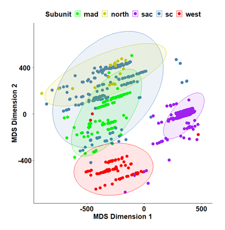
Figure 5: Classical Nonlinear Metric Multidimensional scaling (MDS) showing the distribution, in 2-dimensional space of the distance relationships among Eco-geographic Units (EGU) based on macroscale environmental characteristics. Mad River EGU = mad, Northern Basin EGU = north, Sacramento River = sac, South-Central Basin EGU = sc, and Western Basin = west; colors are matched to Figure 1. Ellipses represent 95% confidence intervals.
Habitat Suitability
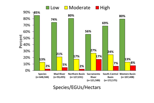
A total of 16,624 random-points (16.5% of 100,000) were identified by selection criteria using the original point- samples for M. churchi. The percentage of random-points selected was mostly consistent in proportion to area each EGU: 1) Mad River (3.7%), 2) Northern Basin (3.6%), 3) Sacramento River (4.1%), 4) South-Central Basin (4.9%), and 5) Western Basin (3.1%). Using these random-point samples, estimates of hypothesized suitable habitat for the species ranged from locations that contained zero suitable habitat to highly suitable habitat (> 19 random-point samples in one grid cell). Similarly, samples from EGU suitability models ranged from zero to 21 random-point samples in one grid cell. The total area of suitable habitat for all EGUs combined totaled ~622009 ha (Figure 6). The percentage of ha in each suitability category varied considerably among EGUs compared to the species HSM (not figured). The Sacramento River was somewhat anomalous in this regard having less Low, more Moderate, and more than twice the total ha of Highly suitable habitat compared to other groups (Figure 7). Overall, bar charts for all groups showed that most habitat consisted of Low suitability (low quality). In total area there were few ha of Moderate or High suitable habitat throughout the range of the species. The Sacramento River, and Western and South-Central basin EGUs had progressively the most highly habitat.
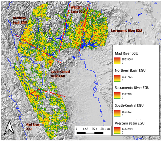
Figure 6: Habitat suitability heatmaps for each Eco-Geographic Unit (EGU) within the geographic range of M. churchi. Suitability ranged from Low = green color, Medium = yellow color, to High = red color. Inset numbers represent the comparative range in hypothesized potential grid-cell density (D.Est.) for snails surrounding each sample site in different colored habitat landscapes.
GAM Regression, Predictors, and Fitted GAM and Random Forest Models
GAM edf values depicting significant driver-D.Est. correlations split between non-linear or highly non-linear (edf > 1, 61.9%, n = 21 comparisons) and linear correlations (edf = 1.0, 38.1%) (Table 6). Inter-group predictor-response relationships varied considerably in the ability to estimate D.Est. statistics. GAM regression showed that D.Est. values for point-samples within the South-Central and Western basin EGUs were primarily correlated with predictors within the Macroscale Climate and Exposure-Distance categories. D.Est. values for point-samples within the Mad River EGU were significantly correlated with covariant predictors within the Exposure-Distance to Stream category, whereas D.Est. values for the Sacramento River EGU were significantly correlated with predictors within the Forest Stand Structure, Mesoscale Climate, and Exposure-Distance to Stream categories and D.Est. values for point-samples within the Northern Basin were significantly associated with predictors within Forest Stand Structure and Mesoscale Climate categories. When all predictor variables were considered in GAM regressions for all groups, the categories of predictor variables significantly correlated with D.Est. where: Macroscale Climate followed by Exposure-Distance to Stream and Forest Stand Structure. GAM regression statistics of driver-D.Est. relationships based on all environmental covariants simultaneously, always produced the highest R2, Dev.Exp., and lowest AIC values across all groups (Table 7).
| Intercept | M. churchi (n = 209) | Mad River (n = 114) | Northern Basin (n = 67) | |||||||||
|---|---|---|---|---|---|---|---|---|---|---|---|---|
| Parametric coefficients | Parametric coefficients | Parametric coefficients | ||||||||||
| Est. | Std.Er. | t-value | P-value | Est. | Std.Er. | t-value | P-value | Est. | Std.Er. | t-value | P-value | |
| 1.12 | 0.06 | 18.5 | 0.001*** | 0.86 | 0.07 | 12.12 | 0.001*** | 0.5 | 0.06 | 7.71 | 0.001*** | |
| Significance of smooth terms | Significance of smooth terms | Significance of smooth terms | ||||||||||
| Variables | edf | Ref.df | GAM-F | P-value | edf | Ref.df | GAM-F | P-value | edf | Ref.df | GAM-F | P-value |
| Forest Stand Structure | ||||||||||||
| CCFA | 1 | 1 | 0.74 | 0.395 | 1 | 1 | 1.56 | 0.214 | 1.85 | 1.97 | 2.69 | 0.105 |
| HCFA | 1 | 1 | 0.38 | 0.534 | 1.1 | 1.19 | 1.42 | 0.196 | 1 | 1 | 2.36 | 0.131 |
| OSTD | 1 | 1 | 1.43 | 0.233 | 1 | 1 | 0.06 | 0.812 | 1.94 | 1.99 | 3.93 | 0.031* |
| TCFA | 1 | 1 | 0.59 | 0.442 | 1 | 1 | 2.48 | 0.119 | 1 | 1 | 2.61 | 0.113 |
| TSIZ | 1 | 1 | 0.32 | 0.574 | 1.87 | 1.98 | 2.93 | 0.051 | 1 | 1 | 4.71 | 0.349 |
| Mesoscale Climate | ||||||||||||
| PASM | 1.9 | 1.99 | 4.61 | 0.009** | 1.64 | 1.87 | 2.33 | 0.072 | 2 | 2 | 8.81 | 0.006** |
| PAWN | 1 | 1 | 2.53 | 0.113 | 1 | 1 | 0.16 | 0.692 | 1.75 | 1.94 | 1.45 | 0.304 |
| TASM | 1 | 1 | 3.54 | 0.690 | 1 | 1 | 0.14 | 0.711 | 1 | 1 | 0.13 | 0.722 |
| TAWN | 2 | 2 | 9.61 | 0.001*** | 1 | 1 | 1.01 | 0.317 | 1 | 1 | 1.11 | 0.297 |
| Exposure-Distance to Nearest Stream | ||||||||||||
| DNST | 1.49 | 1.73 | 1.8 | 0.113 | 1 | 1 | 6.05 | 0.016* | 1.5 | 1.74 | 0.35 | 0.588 |
| ELEV | 1.89 | 1.99 | 3.31 | 0.046* | 1 | 1 | 4.95 | 0.028* | 1 | 1 | 2.12 | 0.152 |
| HLSD | 1 | 1 | 0.11 | 0.739 | 1.07 | 1.13 | 0.01 | 0.981 | 1.24 | 1.43 | 1.59 | 0.315 |
| SLOP | 1 | 1 | 1.05 | 0.308 | 1.54 | 1.79 | 3.02 | 0.039* | 1.68 | 1.9 | 1.75 | 0.256 |
| Intercept | Sacramento River (n = 152) | South-Central Basin (n = 528) | Western Basin (n = 126) | |||||||||
| Parametric coefficients | Parametric coefficients | Parametric coefficients | ||||||||||
| Est. | Std.Er. | t-value | P-value | Est. | Std.Er. | t-value | P-value | Est. | Std.Er. | t-value | P-value | |
| 1.34 | 0.05 | 24.44 | 0.001*** | 0.88 | 0.03 | 25.29 | 0.001*** | 1.28 | 0.07 | 18.43 | 0.001*** | |
| Significance of smooth terms | Significance of smooth terms | Significance of smooth terms |
Table 6: Summary of GAM regression fit statistics for predictors on estimates of grid-cell density (D.E.st.). Comparisons are bas
- Variables edf
- Ref.df
- GAM-F
- P-value edf
- Ref.df
- GAM-F
- P-value edf
- Ref.df
- GAM-F
- P-value
- Forest Stand Structure
- CCFA
- 1.56
- 1.8
- 1.08
- 0.419
- 1
- 1
- 0.02
- 0.885
- 1.9
- 2
- 3.9
- 0.029*
- HCFA
- 1
- 1
- 1.65
- 0.201
- 1
- 1
- 0.01
- 0.924
- 1
- 1
- 2.2
- 0.137
- OSTD
- 1
- 1
- 6.21
- 0.014*
- 1
- 1
- 0.06
- 0.813
- 1
- 1
- 0.1
- 0.701
- TCFA
- 1
- 1
- 2.14
- 0.146
- 1
- 1.01
- 0
- 0.929
- 1
- 1
- 2
- 0.156
- TSIZ
- 1.89
- 1.99
- 4.09
- 0.022*
- 1
- 1.01
- 0.03
- 0.864
- 1
- 1
- 1.6
- 0.215
- Mesoscale Climate
- PASM
- 1
- 1
- 0.36
- 0.55
- 1.79
- 1.96
- 2.07
- 0.152
- 1.8
- 2
- 7.1
- 0.003**
- PAWN
- 1.28
- 1.48
- 3.26
- 0.106
- 1
- 1
- 5.93
- 0.015*
- 1.9
- 2
- 7.5
- 0.002**
- TASM
- 1
- 1
- 1.04
- 0.31
- 1.05
- 1
- 6.96
- 0.009**
- 1
- 1
- 4
- 0.048*
- TAWN
- 1
- 1
- 5.53
- 0.020*
- 1.51
- 1.76
- 1.96
- 0.232
- 1
- 1
- 1.9
- 0.168
- Exposure-Distance to Stream
- DNST
- 1
- 1
- 7.04
- 0.008**
- 1.9
- 1.99
- 3.75
- 0.032*
- 1
- 1
- 0.4
- 0.535
- ELEV
- 1
- 1
- 1.63
- 0.204
- 1
- 1
- 15.21
- 0.001***
- 1.9
- 2
- 4
- 0.025*
- HLSD
- 1.59
- 1.83
- 1.22
- 0.221
- 1
- 1
- 5.06
- 0.025*
- 1
- 1
- 0.3
- 0.568
- SLOP
- 1
- 1
- 3.35
- 0.069
- 1
- 1
- 1.14
- 0.295
- 1
- 1
- 0.1
- 0.725
Table 7: GAM regression models of predictors-driven grid-cell density estimates for the species and EGUs. 1).
| Environmental Variable category | M. churchi | Mad River | Northern Basin | ||||||
|---|---|---|---|---|---|---|---|---|---|
| R2 | Dev.Exp. | AIC | R2 | Dev.Exp. | AIC | R2 | Dev.Exp. | AIC | |
| All variables | 0.13 | 0.29 | 895 | 0.14 | 0.37 | 422 | 0.26 | 0.55 | 178 |
| Forest Stand Structure | 0.04 | 0.06 | 949 | 0.04 | 0.12 | 447 | 0.10 | 0.24 | 198 |
| Mesoscale Climate | 0.12 | 0.21 | 900 | 0.06 | 0.20 | 435 | 0.13 | 0.33 | 183 |
| Exposure-Distance to Stream | 0.07 | 0.15 | 923 | 0.10 | 0.19 | 433 | 0.10 | 0.26 | 190 |
| Environmental Variable category | Sacramento River | South-Central Basin | Western Basin | ||||||
| R2 | Dev.Exp. | AIC | R2 | Dev.Exp. | AIC | R2 | Dev.Exp. | AIC | |
| All variables | 0.31 | 0.52 | 699 | 0.04 | 0.08 | 1900 | 0.09 | 0.27 | 595 |
| Forest Stand Structure | 0.14 | 0.16 | 775 | 0 | 0.01 | 1937 | 0 | 0.04 | 611 |
| Mesoscale Climate | 0.11 | 0.40 | 716 | 0 | 0.01 | 1939 | 0.05 | 0.12 | 596 |
| Exposure-Distance to Stream | 0.09 | 0.26 | 752 | 0.02 | 0.04 | 1908 | 0 | 0.06 | 606 |
Table 8: Summary of GAM regression fit statistics for predictors on estimates of grid-cell density (D.E.st.). Comparisons are bas
Table 7: Summary of GAM regression fit statistics for predictors on estimates of grid-cell density (D.E.st.). Comparisons are based on all variables vs. categories of variables for each group. Environmental categories and variables. *Forest Stand Structure (CCFA = Conifer Cover from Above, HCFA = Hardwood Cover from Above, OSTD = Over-story Tree Diameter, TCFA = Total Tree Cover from Above, TSIZ = Tree Size Class. *Mesoscale Climate (PASM = Average Annual Summer Precipitation (mm), PAWN = Average Annual Winter Precipitation (mm), TASM = Average Annual Summer Temperature (℃), TAWN = Average Annual Winter Temperature (℃). *Exposure-Distance to Stream (DNST = Distance to Nearest Stream (m), ELEV = Elevation, HLSD = Hill-shade, SLOP = Slope). R2 = a measure of correlation between predictions made by the model and actual observations. Dev.Exp. = proportion of null deviance explained; Akaike’s goodness of fit criterion for the regression; variable categories for each regression with the highest fit statistics are bolded.
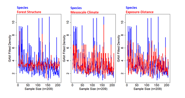
Figure 8: Plots of fitted estimates of density (D.Est) derived from GAM regression versus each environmental predictor category (Forest Stand Structure, Mesoscale Climate, and Exposure-Distance). Coefficients are provided only for M. churchi based on space limitations. The more overlap between blue (species) and red (category) lines the better the fit with the original M. churchi dataset. All plots represent a random subset (21.0%) of the total.
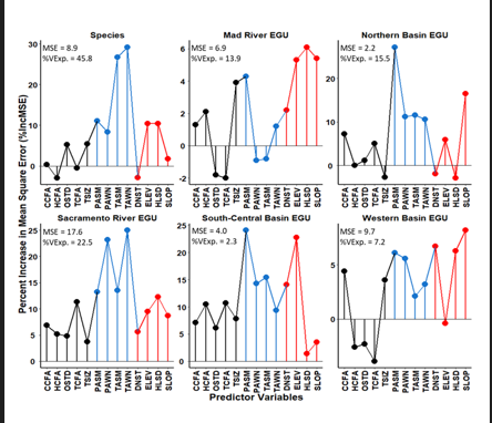
Figure 9: Random forest regression dot-plots of the percent increase in mean square error (%IncMSE), which shows the ability of each predictor variable to estimate density (D.Est.) for each group. %VExp. = percent variance explained and MSE = mean squared error of each model. The closer the MSE value is to zero, the more accurate the model. Predictor color categories: green = Forest Stand Structure, blue = Mesoscale Climate, and orange = Exposure-Distance to Nearest Stream.
Moreover, focusing only on all variables for M. churchi, the Macroscale Climate model followed by the Exposure- Distance to Stream model provided the best suite of driver-D. Est. predictors. Statistically, the species GAM fitted model, based on all variables, was significantly different from covariant predictors within Forest Stand Structure model (F = 5.5, p < 0.001, n = 203) and the Exposure-Distance to Nearest Stream model (F= 2.6, p = 0.004), but not for the Macroscale Climate model (F= 1.7, p = 0.087) (Figure 8). Concordantly, dot-charts of variable importance produced by Random Forest regression [51] (Figure 9) showed that predictor categories with importance values > 10 were: 1) Macroscale Climate followed, Exposure-Distance to Stream, and Forest Stand Structure in sequence. Large %IncMSE values signaled a large difference from randomly permuted variables making the modeled predictors important to the final model. Negative or zero values indicated that driver variables were not predictive enough to be important, as the random variables performed better in the whole model [50, 53, 54]. The proportions of the variance explained (%VExp.) in all models was low, particularly in the South- Central Basin and Western basins. Nonetheless, Kruskal- Wallis non-parametric ANOVA showed a significant overall differences in the values of %IncMSE among all groups ( 2_x_ = 21, p = 0.001, df = 5). And Dunn’s test of post-hoc pairwise comparisons showed that the Sacramento River and South- Central Basin EGUs were significantly different from the Mad River EGU (Z = 3.5, p = 0.002, Z = 3.6, p = 0.003, respectively), and Western Basin EGU (Z = 2.9, p = 0.006, and Z = 3.1, p = 0.006, respectively).
Discussion
Species Versus River-Segregated EGUs
Results of my study highlight the importance of using macroscale distribution models when predicting the distribution and habitat relationships of a wide-ranging species. I show that point-samples of M. churchi and its EGU subpopulations, separated by riverine and associated riparian corridors, followed predominantly east-west and north-south topographic vectors. Riverine-segregated EGUs were significantly different in all biotic and abiotic macroscale habitat characteristics. Ecologically, the most distinct EGU was the Sacramento River. Point-samples in this EGU are found in more arid environs’ downslope within foothill, scrub, and grassland habitats of the Sacramento Valley, compared to upslope montane forest conditions typically found surrounding all other EGUs. The Western Basin EGU was transitional for both up and down slope habitat conditions, whereas the Northern Basin, South- Central Basin, and Mad River EGUs occupied more forested high elevation montane surroundings.
Although M. churchi point-samples were dominated by a diverse assemblage of macroscale forest cover-types and stand structure, combined with physical and other biological attributes, no single or suite of covariant drivers defined suitable macroscale habitat across the range of the species or individual EGUs. Instead, a more robust combination of environmental variables was key to the distribution of point- samples in these groups, as determined by local ecology and topography. My results also show that models consisting of all variables were more “efficient” than models partitioned into individual categories of covariant predictors. Thus, given the macroscale differences in the ecology across the range of M. churchi, it seems logical to consider local heterogeneity among EGUs, on an individual basis, when modeling suitability for purposes of management and conservation planning. Use of a priori disjunct riverine-segregated EGUs, or any other ecological or topographic grouping, to construct a hypothetical HSMs for comparison with M. churchi (as a whole) would therefore, appear to be a logical and ecologically relevant design for modeling potential suitable habitat in wide-ranging taxa [48, 51]).
Density Estimates
Quantification of estimates of grid-cell density, versus environmental predictors, varied considerably between and among the species and EGUs. The most significant GAM-generated regression models portraying predictor-D. Est. relationships were non-linear or strongly non-linear relationships. These driver-response relationships were typical of Macroscale Climate and Exposure-Distance to Stream categories, which were the most important in modeling estimates of D.Est across the range of M. churchi. Detection of non-linearities (threshold responses) in predictor-response relationships is important because they often indicate ecological boundaries (EGUs) that function as critical reference points to avoid or target when making management decisions [52]. Both GAM and Random Forest regression models identified categories and individual variables that were important as covariant predictors of D.Est. Multiple regression of driver-D.Est. relationships based on all environmental covariants simultaneously always produced the highest R2, Dev.Exp., and the lowest AIC values for the species and each intra-species EGU. No individual covariant stood out as most explanatory compared to other attributes evaluated for the species or a particular EGU. These analyses suggests that datasets consisting of all variables were the most informative for use in estimating D.Est. in all groups. Although there was considerable variation in estimates of D.Est. by specific predictors, all regression analyses agreed that the Macroscale Climate category contained the most informative suite of predictors across groups, followed by the Exposure-Distance to Nearest Stream models. This
conclusion was further substantiated by Random Forest model statistics.
For M. churchi, all macroscale models were rather inefficient at predicting D.Est. As such, use of grid-cells in combination with random points, may not be the best method to estimate density or particularly informative at a landscape-level, even though estimates were based on selection criteria derived from the original point-samples. A better approach may be to gather density data during ground surveys. However, this creates logistical issues, particularly in species with broad geographic ranges, and in areas of inaccessible and rugged terrain. Moreover, detailed, and wide-spread density estimates of snails are rarely gathered and less frequently reported.
Also, because terrestrial exothermic snails are small, I would expect some sensitivity to climate (hot temperatures) and hence, the importance of microclimate in mitigating summer heat. However, the sites described in my study are mostly moderately to heavily forested. This means that the ecological signal of microclimatic cooling provided by closeness to streams could be blurred since a large portion of the study area was under dense canopy. Thus, complementary sampling at more proximate scales (microhabitat) will likely be a high priority during future sampling, in combination and comparison with macroscale-dependent habitat suitability delineated at the geographic level of the focal-species range.
Mapping of Habitat Suitability Models
My use of combined minimum values as selection criteria for input into the HSM provided a simple way to select macroscale attributes without making post hoc decisions as to which macroscale attribute(s) provided the greatest potential habitat for the species. This was because no single variable or conspicuous suite of variables explained the greatest amount of variance among point-samples. Further, use of a small subset of variables might not capture unique macroscale environmental variance typical of some riverine- segregated M. churchi, as there were many significant univariate differences between and among EGUs.
Geographic variance in the area of suitable macrohabitat illustrated in heatmaps was widely distributed throughout the range of M. churchi. For all EGUs availability of High or Moderate quality habitat was low. At the scale of the landscape these coarse-grained heatmaps may appear to lack sufficient detail about suitability at the ground level, given that climatic variables were at or above-canopy levels and interpolated from distant weather stations. Yet, when viewed at more proximate scales (overlayed onto specific project sites), the functionality of these HSM maps can provide a greater understanding of the locations of underlying site-specific characteristics at a local level (topography, exposure, forest cover-type, hydrology). Early on, this coarse-grained level of detail is particularly important when focusing on suitable microhabitat for: 1) assessment, 2) enhancement of low- moderately suitable habitat, 3) relocation and transplanting of at-risk species based on accompanying population genetic information, and 4) management and planning purposes. Initially I estimated the geographic range of M. churchi to be ~11800 km2 based on the total area encompassed by all documented point-samples. Previous modeling estimated the range of the species at ~15795 km2 based on univariate comparisons defined by 5% probability contours for 1718 random samples [1] and a map produced by use of theoretical hierarchical Bayesian spatial modeling [53]. Yet a better estimate for the range of M. churchi may be estimated using the total area encompassed by all suitable habitat categories for all EGUs (~6220 km2). Surprisingly, the total area of potentially suitable habitat modeled by individual EGUs was much more widely distributed throughout the range of M. churchi than I expected. Nonetheless, for M. churchi there are still large areas that have not been sampled, and likely will not be surveyed both within and outside the Greater Trinity Basin. In reference to the Klamath Biological Region the sample size used in my analysis was the largest, most ecologically diverse, and geographically widespread of any conifer-hardwood-dwelling gastropod yet studied.
Potential Limitations to Sampling for Modeling Suitability
The occurrence of a species in a landscape is a function of numerous factors, each influential at different spatial scales. Evaluating a species distribution by use of multiscale models can improve the predictive ability of the design compared to single-scale models [55]. In suitability modeling selecting the most appropriate scale-dependent predictors and standardizing variables of different scales are important because use of predictors at wrong spatial scales can significantly bias results [54]. These issues can lead to overestimating a species preference for habitat and misleading conclusions regarding the current and future status, location, and management of a population [48]. Additionally, there are several other factors that should be considered when attempting to estimate how well HSMs depict species’ habitat preferences. For example, broad-scale patterns derived from spatial models may be sensitive to: 1) sample size, 2) sampling random-point datasets based on presence and/or absence data, and/or 3) un-surveyed portions of the species range (underestimating a species range).
For example, it was hypothesized that a small number of point-samples, if randomly obtained, may be sufficient to adequately describe species-specific ecological affinities among forest-dwelling terrestrial gastropod communities within late-successional forest ecosystems [1]. Yet the potential always exists for a small number of “random samples” to miss local variation across a region if not representative of that region. This is particularly problematic when organisms are not distributed randomly but are dispersed over a large geographic area with complex habitat heterogeneity, resulting in missed information concerning diversity and acclimatization (specialization) of populations to local environmental variables. Nonetheless, by greatly increasing the sample size of point-samples and density estimates across range of the species, use of random point sampling and grid-cell density estimation would likely not be necessary.
Potential for genetic differentiation
Another complicating factor that cannot be underestimated, but is rarely addressed in suitability analyses, is the presence of potentially unknown morphologically cryptic and ecologically syntopic species at or below the species-level, waiting to be unmasked by use of modern molecular techniques (DNA barcoding, microsatellite markers [17, 56, 57]. It is well established that animals, particularly ectotherms [58, 59], can show morphological differentiation (banding patterns and coloration) and genetic structuring at small spatial scales as a function of the role of physical barriers in promoting population and genetic divergence [60, 61, 62, 63]. This is an elusive problem given the logistical difficulty of surveying geographically and topographically complex, and largely remote landscapes (river systems, mountain ranges) potentially facilitating significant genetic divergence in allopatric populations, at or below the species-level. This consideration may also apply to other regionally complex molluscan faunas that contain morphologically cryptic and ecological equivalent land snail taxa.
For instance, several major river systems within the Trinity Basin were found to be associated with genetic and taxonomic differentiation in M. setosa [17]. Subclade (= subspecies taxonomy) differentiation among populations of forest-dwelling M. setosa occurred within the middle portion of the Greater Trinity Basin, concordant with positioning of major riverine corridors [17]. In M. setosa, genetic and systematic differentiation was based largely on a north- south latitudinal gradient, which includes separation of point-samples by the Trinity River and the South Fork of the Trinity River. Importantly, these same rivers also interrupt the distribution of M. churchi. However, except for M. setosa, detailed comparative genetic and ecological studies of the relationships among allopatric populations and sympatric assemblages of terrestrial gastropods remains largely undocumented within the Klamath Biological Region.
Given that significant habitat conditions exist between riverine-segregated EGUs of M. churchi, in combination with topographic and geographic diversity, the potential for allopatric divergence in some populations, particularly in more arid regions, is highly plausible.
Also, prior to 2002 there were virtually no comprehensive range-wide molecular DNA analyses of species-level relationships among any taxa within the genus Monadenia. Molecular analyses are rudimentary with no assessment of molecular variation among populations or within any taxon or species complex [64]. Monadenia setosa was not identified definitively as a distinct species, with five subspecies separated by river systems, until 18 years later [17]. Although popular in phylogenetic analyses [64], use of only a few random point-samples generally does not encompass the full genetic uniqueness of a species-complex. This is especially true when coupled with an expansive landscape-level geographic diversity and a diverse ecological and biogeographic history. Thus, sampling of > 25 individuals may be necessary for some species exhibiting widespread distribution patterns within these kinds of landscapes [57, 58]. Lastly, as a function of molecular DNA and phylogenetic out-group analysis, the Sierra Sideband snail (Monadenia mormonum) was hypothesized to be the sister-taxon of M. churchi [17]. This development provides strong justification for additional geographic sampling in combination with molecular DNA investigations into the phylogenetic and taxonomic relationships of M. churchi versus M. mormonum. The Sierra sideband is found on the eastside of the Sacramento River valley along the Sierra Nevada escarpment that includes several central Sierra Nevada counties. Modenia mormonum is undoubtedly linked evolutionarily to other woodland- and forest-dwelling species in the genus, which are distributed southward within the Sierra Nevada cordilleran ecozone. Future genetic analyses could potentially facilitate discovery of directional phylogenetic and historical biogeographic relationships in the context of both the Sierra Nevada and the north-central coast range of California for these two species and their generic lineages.
Management Recommendations
Processes that determine the distribution of a species occur at multiple spatial scales [65, 66]. My study provides a baseline for assessment, evaluation, and management of broad-scale and local environmental trends in the geographic distribution of Church’s sideband. For M. churchi, M. setosa, and other similar taxa in the region and elsewhere across California, I recommend that management and conservation of mollusk communities within the Klamath Bioregion and Serra Nevada cordillera follow a multiscale format that combines macroscale and site-specific population-level assessments of suitable habitat throughout the range of each focal taxon [17, 22]. Complementing this scale-dependent strategy requires use of regression analyses to evaluate the strength of predictor-response relationships in estimating density or some other reproductive output. This is because the effects of individual versus the collective “synergistic” or “threshold” characteristics of multivariate models likely have differential influence on the response variable. Use of a landscape-level approach combined with more proximate scales of resolution (microscale) within preferred habitat, and the application of molecular screening of disjunct populations can: 1) provide species-specific baselines, 2) assist in evaluating the most appropriate scale-dependent HSM to address spatial heterogeneity and ecological diversity, 3) provide a more thorough understanding of life history requirements, 4) allow estimates of density and reproductive potential across the landscape, and 5) facilitate a more focused and efficient pathway for future management and conservation of forest-dwelling mollusk communities.
Conflict of Interest
The author declares no conflict of interest
Acknowledgment
I am grateful to S. Dymond for providing clarifying comments on watershed issues. I am also grateful to several anonymous reviewers for providing constructive editorial comments and suggestions on an earlier version of this document.
References
-
Dunk JR, Zielinski WJ, Preisler HK (2004) Predicting the occurrence of rare mollusks in northern California forests. Ecological Applications 14(3): 713-729.
-
Sullivan RM (2022) Microhabitat characteristics and management of the Trinity bristle snail in the Greater Trinity Basin of northern California. California Fish and Wildlife Journal 108: e3.
-
Cameron RAD (1986) Environment and diversities of forest snail faunas from coastal British Columbia. Malacologia 27(2): 341-155.
-
Furnish J, Burke T, Weasma T, Applegarth J, Duncan N, et al. (1997) Survey protocol for terrestrial mollusk species from the northwest forest plan, draft version 2.0. USDA, USFS and BLM.
-
Duncan N, Burke TE, Dowlan S, Hohenlohe P (2003) Survey protocol for survey and manage of terrestrial mollusks species from the Northwest Forest Plan. Version 3.0, pp: 1-70.
-
Foster AD, Ziegltrum J (2013) Northwest Science 83: 243-256.
-
Puig-Gironès R, Santos X, Bros V (2023) Temporal differences in snail diversity responses to wildfires and salvage logging. Environmental Conservation 50(1): 40- 49.
-
Hanna GD, AG Smith (1933) Two new species of _Monadenia_ from northern California. The Nautilus 46: 79-86.
-
Talmadge RR (1952) A bristled _Monadenia_ from California. The Nautilus 66: 47-50.
-
Frest T, Jerrence J, Johannes EJ (1993) Mollusc species of special concern within the range of the Northern Spotted Owl. Deixis Consultants, Final Report. Unpublished report prepared for the Forest Ecosystem Management Working Group, USDA Forest Service, Pacific Northwest Region, Portland.
-
Burke TE, Applegarth JS, Weasma TR (1999) Management recommendations for survey and manage terrestrial mollusks. In: 2nd (Edn.), United States Department of Agriculture, Forest Service, Pacific Northwest Region, Portland, Oregon.
-
Zhivotovsky L (2016) Population structure of species: Eco-geographic units and genetic differentiation between populations. Russian Journal of Marine Biology 42(5): 373-382.
-
Welsh HH (1994) Bioregions: An ecological and evolutionary perspective and a proposal for California. Calif Fish and Game 80(3): 97-124.
-
Munz P, Keck DD (1959) A California Flora. Science 131(3405): 982.
-
Barrett JG (1966) Climate of Trinity County. United States Department of Agriculture Soil Conservation Service, Redding, CA.
-
Shilling F, Sommarstrom S, Kattelmann R, Washburn B, Florsheim J, et al. (2005) California Watershed Assessment Manual. California Resources Agency and the California Bay-Delta Authority 1: 1-248.
-
Sullivan RM (2021) Phylogenetic relationships among subclades within the Trinity bristle snail species complex, riverine barriers, and re-classification. California Fish and Wildlife 2021(CESA S): 107-145.
-
Roth B, Pressley PH (1986) Observations on the range and natural history of _Monadenia setosa_ (Gastropoda: Pulmonate) in the Klamath Mountains, California, and the taxonomy of some related species. The Veliger 29: 169-182.
-
Martin K, M Sommer M (2004) Relationships between land snail assemblage patterns and soil properties in temperate-humid forest ecosystems. Journal of Biogeography 31(4): 531-545.
-
Gotmark F, Proschwitch VT, Niklas F (2008) Are small sedentary species affected by habitat fragmentation? Local vs landscape factors predicting species richness and composition of land molluscs in Swedish conservation forests. Journal of Biogeography 35(6): 1062-1076.
-
Raheem DC, Naggs F, Preece RC, Mapatuna Y, Kariyawasam L, et al. (2008) Structure and conservation of Sri Lankan land-snail assemblages in fragmented lowland rainforest and village home gardens. Journal of Applied Ecology 45(4): 1019-1028.
-
White P, Kimerling AJ, Overton WS (1992) Cartographic and geometric components of a global sampling design for environmental monitoring. Cartography and Geographic Information Systems 19(1): 5-22.
-
Molina R, McKenzie D, Lesher R, Ford J, Alegria J, et al. (2003) Strategic survey framework for the northwest forest plan survey and manage program. United States Department of Agriculture Forest Service, Pacific Northwest Research Station, General Technical Report PNW-GTR-573, pp: 1-44.
-
United States Department of the Interior, USFS (1981) CALVEG: A Classification of California Vegetation. Pacific Southwest Region, Regional Ecology Group, San Francisco CA, USA.
-
Airola DA (1988) A guide to the California wildlife habitat relationships system. State of California, Resources Agency, Sacramento, CA, pp: 166.
-
Mayer KE, Laudenslayer WF (1988) A guide to the wildlife habitats of California. State of California, Resources Agency, Department of Fish and Game, Sacramento, California.
-
Garrison BA, Parisi MD, Hunting KW, Giles TA, McNerney JT, et al. (2002) Training manual for California Wildlife Habitat Relationships System CWHR database version 8.0. Ninth edition. California Wildlife Habitat Relationships Program, California Department of Fish and Game, Sacramento, CA, USA.
-
PRISM (2024) Northwest Alliance for Computational Science and Engineering. Oregon State University, Corvallis, OR, USA.
-
Daly C, Halbleib M, Smith JI, Gibson PW, Matthew KW, et al. (2008) Physiographically-sensitive mapping of temperature and precipitation across the conterminous United States. International Journal of Climatology 28(15): 2031-2064.
-
Helms J (1998) The Dictionary of Forestry. Society of American Foresters, Washington DC, USA, pp: 210.
-
Curtis RO, Marshall DD (2000) Why quadratic mean diameter?. Western Journal of Applied Forestry 15(3): 137-139.
-
Daly C, Neilson RP, Phillips DJ (1994) A statistical- topographic model for mapping climatological precipitation over mountainous terrain. Journal of Applied Meteorology 33(2): 140-158.
-
Burrough PA, McDonnell RA (1998) Principles of geographical information systems. Oxford University Press, Oxford, England, UK.
-
Breiman L (2001) Random forests. Machine Learning 45(1): 5-32.
-
Breiman L (2001) Manual on setting up, using, and understanding random forests V3.1. US Documents pp: 1-29.
-
Demaine E, Hesterberg A, Koehler F, Lynch J, Urschel J (2021) Multidimensional scaling: approximation and complexity. Proceedings of the 38th International Conference on Machine Learning PMLR 139.
-
Wood SN (2011) Fast stable restricted maximum likelihood and marginal likelihood estimation of semiparametric generalized linear models. Journal of the Royal Statistical Society 73(1): 3-36.
-
Hastie T, Tibshirani RJ (1990) Generalized additive models. 1st (Edn.), Chapman and Hall, London, UK.
-
Madsen H, Thyregod P (2011) An introduction to general and generalized linear models. In: 4th (Edn.), Chapman and Hall/CRC, Boca Raton, Florida.
-
Wood SN, Pya N, Saefken B (2016) Smoothing parameter and model selection for general smooth models. Journal of the American Statistical Association 111(516): 1548- 1575.
-
Warren DL, Glor RE, Turelli M (2008) Environmental niche equivalency versus conservatism: Quantitative approaches to niche evolution. Evolution 62(11): 2868- 2883.
-
Thomasma LE, Drummer TD, Peterson RO (1991) Testing the habitat suitability index model for the fisher. Wildlife Society Bulletin 19(3): 291-297.
-
Bender LC, Roloff GL, Haufler JB (1996) Evaluating confidence intervals for habitat suitability models. Wildlife Society Bulletin 24(2): 347-352.
-
Brooks RP (1997) Improving habitat suitability index models. Wildlife Society Bulletin 25(1): 163-167.
-
Roloff GJ, Kernohan BJ (1999) Evaluating reliability of habitat suitability index models. Wildlife Society Bulletin 27(4): 973- 985.
-
Runnebaum J, Guan L, Cao J, O’Brien L, Chen Y (2018) Habitat suitability modeling based on a spatiotemporal model: An example for cusk in the Gulf of Maine. Canadian Journal of Fisheries and Aquatic Sciences 75 (11): 1784-1797.
-
Chang JH, Chen Y, Halteman W, Wilson C (2016) Roles of spatial scale in quantifying stock-recruitment relationships for American lobsters in the inshore Gulf of Maine. Canadian Journal of Fisheries and Aquatic Sciences 73(6): 885-909.
-
Behan JT, Hodgdon CT, Chen Y (2022) Scale-dependent assumptions influence habitat suitability estimates for the American lobster (_Homarus americanus_): Implications for a changing Gulf of Maine. Ecological Modelling 470: 1-10.
-
Valavi R, Elith J, Lahoz-Monfort JJ, Guillera-Arroita G (2021) Modelling species presence-only data with random forests. Ecography 44(12): 1731-1742.
-
Kuhn M, Egert B, Neumann S, Steinbek C (2008) Building blocks for automated elucidation of metabolites: machine learning methods for NMR prediction. BMC Bioinformatics 9(1): 400.
-
Fotheringham AS, Brunsdon C, Charlton M (2002) Geographically weighted regression: the analysis of spatially varying relationships. Geographical analysis 35(3): 272-275.
-
Zhivotovsky LA, Shitova MV, Rakitskaya TA, Rubtsova GA, Afanasyev KI, et al. (2021) Ecogeographic units and management units of Chum Salmon _Oncorhynchus_ _keta_ of the Amur Zoogeographic Province. Journal of Ichthyology 61: 585-593.
-
Carrol C, Johnson DS, Dunk JR, Zielinski WJ (2010) Hierarchical Bayesian spatial models for multispecies conservation planning and monitoring. Conservation Biology 24(6): 1538-1548.
-
Bradter U, Kunin WE, Altringham JD, Thom TJ, Benton TG (2013) Identifying appropriate spatial scales of predictors in species distribution models with the random forest algorithm. Methods Ecological Evolution 4(2): 167-174.
-
Cunningham MA, Johnson JA (2006) Proximate and landscape factors influence grassland bird distributions. Ecological Applications 16(3): 1062-1075.
-
Becker S, Hanner R, Steinke D (2011) Five years of FISH‐ BOL: Brief status report. Mitochondrial DNA 22(1S): 3-9.
-
Steinke D, Hanner R (2011) The FISH‐BOL collaborators’ protocol. Mitochondrial DNA 22(1S): 10-14.
-
Català C, Bros V, Castelltort X, Santos X, Pascual M (2021) Deep genetic structure at a small spatial scale in the endangered land snail _Xerocrassa montserratensis_. Scientific Reports 11(1): 1-10.
-
Buono V, Bissattini AM, Davoli F, Chiara M, Nadia M, Leonardo V (2023) Fine-scale spatial genetic structure and dispersal among Italian smooth newt populations in a rural landscape. Scientific Reports 13: 1-13.
-
Jones JS , Selander RK, Schnell DG (1980) Patterns of morphological and molecular polymorphism in the land snail _Cepaea nemoralis_. Biological Journal of the Linnean Society 14(3-4): 359-387.
-
Davison A, Clarke B (2000) History or current selection? A molecular analysis of ‘area effects’ in the land snail _Cepaea nemoralis_. Proceedings of the Royal Society B 267(1451): 1399-1405.
-
Garrett LJH, Myatt JP, Sadler JP, Dawson DA, Hipperson H, et al. (2020) Spatio-temporal processes drive fine-scale genetic structure in an otherwise panmictic seabird population. Scientific Reports 10: 20725.
-
Major RE, Ewart KM, Portelli DJ, King A, Tsang LA, et al. (2021) Islands within islands: genetic structuring at small spatial scales has implications for long-term persistence of a threatened species. Animal Conservation 24(1): 95-107.
-
Cordero AM, Lindberg DL (2002) Molecular phylogeny of some land snails of the clades _Monadenia_ and _Helminthoglypta_ in southern Oregon and Northern California. Final Report submitted to Bureau of Land Management District Office, Roseburg District Office, Roseburg, Oregon.
-
Thogmartin WE, Knutson MG (2007) Scaling local species-habitat relations to the larger landscape with a hierarchical spatial count model. Landscape Ecology 22: 61-75.
-
Wiens JA (1989) Spatial scaling in ecology. Functional Ecology 3(4): 385-397.
- Mitochondrial Bio-Logistics: Steering Co-Enzyme Q10 and Lycopene Synergies within the Science 4.0 Bio-OS Framework
- Hymenoptera Specimens from the Caño Negro Wetland, of the National Museum Collection, Costa Rica
- Science 4.0: Comprehensive Architecture of the Biological Operating System (Bio-OS) A Framework for Systemic Resilience and Industrialized Bio-Governance
- Rabbit on, or Hare Back? Understanding Climate Change
- Clinical Validation of Science 4.0: Flow Steering and Epigenetic Drift Inversion on a 76-Year-Old Hybrid System
- Seeds Planted by another Mind