Breast Cancer Early Detection Comparison with Deep Learning and Machine Learning Models: A Case of Study
Breast cancer is one of the most widespread in the female population, being able to predict its developments and capturing the inputs of the onset of the disease is one of the main objectives that science is pursuing. Clinical Decision Support Systems (CDSS) in recent decades are extensively using these technological tools, such as Machine Learning (ML) and Deep Learning (DL). In this paper, two of the main methods of these subset of AI are compared: an ensemble-type algorithm, XGBoost (or Extreme Gradient Boosting) and a deep neural network (DNN) are applied to the data of a study conducted on an Indonesian population. The results obtained are very interesting as despite being tabular, binary categorical and multiclass data, the DNN model achieves performance and results much higher than the well-known XGB used in literature for data of this type.
Introduction
The following section discusses the motivation and purpose of the work in order to direct the reader from the beginning to understand the methods used, the data used and the purposes pursued by the study of the real case analyzed in the following sections.
Motivation
The interest created around deep learning, a subfield of artificial intelligence techniques which aim to emulate the cognitive behavior of the human and animal brain (ie. with Convolutional Neural Networks), has produced a multitude of works in the field computer vision (CV) for the study of phenomena related to cancer, through the analysis of radiographs and images more generally. The precision and accuracy with which these methods work, thanks also to the development of the computational power, has meant that today they are widely used and discussed, also due to their lack of ”transparency”. In this work, more than demonstrating once again the performance capacity of these methods, such as deep neural networks, we tried to show by comparing two types of methods different but belonging to the same area, namely artificial intelligence that within it includes machine learning and deep learning a greater effort has been made: evaluate on structured data, in tabular format, and show that despite classical methods such as ensembles that are known to work better on structured data, deep learning still remains the default state-of-the-art benchmark. The work is composed as follows: after the reasons introduced follows a part that defines the purpose of the work, in section 2 instead we propose a general overview of what deep learning is and on the main architectures and then in the next subsection to present the state of the art on the works for which deep learning it has been used in cancer classification and analysis. Section 3 collects the part relating to the analyzed data, the modeling methods used and the results obtained from the models, with a focus on features importance and interpretation of the results. In the last part (section 4) final remarks and conclusions. As a demonstration of the value and robustness of the solution adopted, a real case study involving a population is analyzed reference on which to predict the development of breast cancer disease.
Purpose
From the scientific works published and mentioned in the next section it is easy to notice almost all the works in the majority of cases they concern the application of deep learning techniques on images, whether they are radiography or images in general. Does this make sense as the extraction of features from images generates very large dimensionality and a massive amount of data for which it is good to use convolutional neural networks, for example. In this work instead, which concerns the possibility of applying these techniques to prevention of breast cancer, data are used that are not images, rather they are so-called tabular data: these data in fact did not require particular manipulations and this is consistent as they were collected through a questionnaire. The data used come from a so-called case-control study and generally these data are used only for statistical purposes to extract relationships and correlations, to infer data and draw conclusions in terms of study on a specific population to extend the assumptions made to sampled populations. The aim is therefore to evaluate the application of deep learning techniques to tabular data rather than models in general more performing such as XGBoost or Logistic regression. For this purpose, two approaches are compared in the modeling phase: the classical one for tabular data through the application of an XGBoost ensemble and the one of a multilayer neural network. The first method certainly offers greater interpretability and transparency, compared to the so called ”black boxes”, as well as responding to a series of different computational requirements with respect to the expenditure of computational resources such as GPU in the application of neural networks, but for which in this specific work the problem does not arise, as the input instance is very small: we are talking about 400 samples and in the order of tens for the number of columns. It is not even that simple, and it would be superficial, to think, however, that since the data are tabular, the a priori performances of classical methods such as XGBoost are superior: the data collected for the questionnaire, however, they are categorical, multiclass data and their engineering, through encoding or dummy transformation, however, makes the training of the algorithms complex. From the comparison it emerges that in any case both one and the other method produce good results, being the field of application however of a clinical type, having interpretable and transparent tools, however, remains an advantage that to date the neural networks on tabular data do not allow, contrary to methods developed for computer vision in image analysis. The tradeoff therefore remains whether to choose interpretability or precision.
Background
This section provides the technical and methodological tools to the reader to understand the scope of deep learning to problems related to breast cancer prediction and analysis: the state of the art and the most common deep neural network architectures are presented. In order to have a clearer view of the context and more recent literary references.
Deep learning: Architectures and Models
The escalation of artificial intelligence in recent years, in every field of application has become disruptive and preponderant. Deep learning, a branch of machine learning, which through the application of complex mathematical structures, such as neural networks, which emulate human cognitive behavior, is able to extract complex patterns and structures in data and is able to classify or predict phenomena very accurately [1, 2, 3, 4, 5, 6, 7, 8, 9, 10, 11, 12, 13, 14, 15, 16, 17, 18, 19, 20, 21, 22]. This accuracy, however, is affected by the interpretability and explainability of the results: these methods are in fact considered ”black boxes” even if in recent years a new branch of AI so-called Explainable AI (XAI) has been born. The application of deep learning, of neural networks more generally, is very broad: from the analysis of natural language, Natural Language Processing (NLP) to audio and speech recognition as well as image and video analysis [23, 24, 25, 26, 27, 28, 29, 30, 31, 32, 33]. Artificial neural networks have at least 70 years of history as a mathematical formulation, but their widespread use has been made possible by the evolution of computers and computing power [34, 35, 36], and above all from the massive production of data which in recent years has seen an exponential growth. The ability of artificial neural networks is to extract features automatically without the need to have domain expertise as in the most common problems in which machine learning is applied: there are different types of neural networks, from the simplest, that is the Percerptron: this model was proposed by Minsky-Papert as one of the simplest models, also known as TLU (logical unit of threshold) [37] (Figure 1).
![Figure 1: Classical ANN architectures [38].](/fulltextimages/9560/fig_1.png)
The model takes as input the instances that are weighted and applies an activation function to obtain the output as the final result. A more complex version is the Multilayer perceptron one which has three or more layers. It is used to classify data that cannot be separated linearly. It is a type of fully connected artificial neural network. This is because every single node in a tier is connected to every node in the next tier. Usually the activation function of a multilayer perceptron is nonlinear (mainly hyperbolic tangent or logistic function). A more advanced model is that of the Feed Forward neural network, in which the input data moves in one direction only, passing through a layer of nodes and exiting through output nodes. The number of (hidden) levels depends on the complexity of the cost function being defined. It has one-way forward propagation but no backpropagation. An activation function is powered by inputs which are multiplied by weights. The neuron is activated if it is above the threshold and the neuron produces 1 or 0 otherwise. Over time several types have been developed including Convolutional neural networks (CNNs) which use a variation of the multilayer perceptron 3. A CNN contains one or more convolutional layers. It gets its name from a linear mathematical operation between matrices called convolution. CNN has multiple levels; including the convolutional layer, the non-linearity layer, the pooling layer and the fully connected layer. Convolutional and fully connected levels have parameters but pooling and non-linearity levels do not have parameters. These levels can be completely interconnected or grouped. Before passing the obtained output from the previous level to the next, the convolutional level uses a convolutional operation on the input, which is used to progressively extract higher level representations. Another widely used type of neural network is that Recurrent is a type of artificial neural network in which the output of a particular layer is saved and returned to the input 2 (Figure 2).
![Figure 2: RNN standard architectures [39].](/fulltextimages/9560/fig_2.png)
Similarly to the feedforward network the first layer is formed in the same way. That is, with the sum of the weighted product of the input of the characteristics. In the following levels, instead, the recurrence process begins between the output that becomes the input in the next step. From each time step to the next, each node will store the information it had acquired in the previous step. Each node acts as a memory cell when calculating for performing operations. The neural network starts with propagating forward, but it remembers the information it may need to use in the next step. The
concept is that if the network makes an incorrect prediction the system auto learns and improves the prediction during back propagation (Figure 3).
![Figure 3: CNN architectures [37].](/fulltextimages/9560/fig_3.png)
Deep Learning and XGBoost for Cancer Prediction
The application of deep learning to cancer screening is a very widespread topic in the literature, several works have been proposed in recent years, especially with the evolution of calculation systems that actually allow the massive processing of data: the methods used most in fact are those based on convolutional architectures since the data with which to train the topics are mainly images, such as radiographs. Preventive screening and cancer diagnosis in recent years have focused on problems related to cervical cancer, lung cancer, prostate and above all breast cancer [14, 15, 16, 17, 18, 19, 20, 21]. The work of Wang, et al. [1] presents a very interesting method as it combines two different machine learning or artificial intelligence techniques more generally: the first is the improvement of the data available, through the application of a C-mean Fuzzy clustering on the CT images of the breast cancer of the population examined in order to optimize the image (CBIS-DDSM Image Library and MIAS Image Library The British Image Analysis Association); subsequently they use a convolutional neural network (CNN). The authors state that this combined method produces a better classification for breast cancer screening. The authors Chen, et al. [2] present an interesting work for cervical cancer screening, proposing a method based on three modules: the first that segments the cervical cells that extracts the cellular images in an image, to be considered as a features extractor, then the core module, which through a VGG (compact visual geometry group (VGG) network called Compact (VGG) performs the cell classification part and the last module, the visualization module, which helps the clinical operator in the final diagnosis of the screening. The proposed system is called CytoBrain and was trained on a sample of 198,952 images from 2,312 adult women. Becker, et al. [3] propose a study on the use of generic deep learning software (DLS) in order to classify breast cancer on ultrasound images and compare the results obtained with the human counterpart, i.e. clinical operators, thus studying the ability of an AI system to support diagnosis and automate the screening process. The authors use data from breast ultrasound examinations from January 1, 2014 to December 31, 2014. The DLS was trained with 70% (train set) of the images and the remaining 30% was used to validate performance (validation set). Subsequently the DLS algorithm was compared with the judgment of three readers who also evaluated the validation set. The training time was 7 minutes (DLS). The evaluation time for the test dataset was 3.7 seconds (DLS) and 28, 22, and 25 minutes for human readers (decreasing experience). The authors conclude that DLS can help diagnose cancer on ultrasound breast images with accuracy equal to that of radiologists, learning faster than a human reader without prior experience. This method is certainly promising as it drastically reduces diagnosis times. Ji et al. to the study artificial intelligence methods for diagnosing disease progression, evaluating machine learning (ML) in order to be able to distinguish between malignant and benign breast lesions on a clinical magnetic resonance imaging (MRI) dataset. The study was carried out on 1483 patients with breast cancer and 496 benign patients who underwent MRI exams between February 2015 and October 2017; patients were separated into a training dataset (years 2015 and 2016; 1444 cases) and a test dataset (year 2017; 535 cases). The process first sees a screening by the radiologist who indicates the lesion and subsequently, the radiomic features are automatically extracted, used for the training of the SVM. The authors obtain promising results, in terms of AUC (Area Under Curve): the trained predictive model produced an AUC value of 0.89 with confidence intervals (CI) 95% CI: 0.858, 0.922 on the test image set Antonelli, et. al. [5] they too propose a study that aims to compare whether a classifier based on machine learning (ML) is comparable in terms of precision and accuracy, to the medical opinion of experts. The study investigates whether ML algorithms for the transition zone (TZ) and peripheral zone (PZ) can correctly classify prostate cancers in those with or without a Gleason 4 component (binary classification) and compare the performance with three radiologists. Data refer to the period between 2012 and 2015. Index lesions from 164 men (119 PZ, 45 TZ) were analyzed. Quantitative MRI and clinical features were used, and area-specific machine learning classifiers were built. Models were validated using fivefold cross-validation and a temporarily separate patient cohort. The authors get good results: the best classifier for PZ trained with prostate specific antigen density, apparent diffusion coefficient (ADC), and maximum improvement (ME) on DCE-MRI achieved an ROC area under the curve (AUC) of 0.83 by five iterations of cross-validation. The diagnostic sensitivity at 50% of the specificity threshold was greater for the best PZ model (0.93) than the mean sensitivity of the three radiologists (0.72). The best model for the TZ, on the other hand, was trained on ADC and ME to obtain an AUC of 0.75 after a cross validation also of five iterations: this allowed a greater diagnostic sensitivity at 50% of the specificity threshold (0.88) compared to to the average sensitivity of the three radiologists (0.82). The authors conclude that also in this case the use of ML techniques has led to a more efficient prediction and diagnosis than that of man, namely the three radiologists. Remaining in the field of image analysis for cancer detection more generally, Zhang, et al. [6] applying a convolutional neural network (CNN) training on 1660 SLIM images (spatial light interference microscopy) of colon glands and validating on 144 glands obtained an accuracy of 98% (validation set) and 99% (test set), resulting in the accuracy of the benign classification compared to 97% cancer in terms of AUC. The authors also believe that the SLIM full-slide scanner combined with deep learning may prove invaluable as a pre- screening method, saving time in the diagnosis phase. The works seen so far and the classic Deep learning algorithms that we have seen working, work mainly on images, through computer vision techniques based on CNN for example: it is not the only one method that can be pursued obviously. The study by Zhang, et al. [7] proposes a method based on Natural Language Processing, which however makes use of architectures based on neural networks. This work analyzes computed tomography (CT) reports that record a large volume of information about patients’ conditions. The authors investigate a new deep learning method to extract entities from Chinese CT reports for lung cancer screening and TNM staging. The approach relies on the recognition of named entities, namely the BERT-based BiLSTM-Transformer network (BERT-BTN) with pre-training, to extract clinical entities for lung cancer screening and staging. In this case BERT is applied to learn the deep semantic representations of the characters, then a Transformer layer is added to the long short term memory level in order to acquire the global dependencies between the characters. The data supporting the evidence obtained by the algorithm is based on a clinical data set containing 359 CT reports collected by the ”Department of Thoracic Surgery II of the Peking University Oncology Hospital”. The experimental results present a macro-F1 score of 85.7% improving the results obtained by up to 8% compared to models such as BERT-BTN, BERT- LSTM, BERT-fine-tune, BERT-Transformer, FastText-BTN, FastText-BiLSTM and FastText-Transformer, respectively. Regarding the use of Extreme Gradient Boosting (XGBoost) in the predictive treatment of breast cancer, several papers have recently been published: in the work of breast cancer is modeled by means of an XGBoost, where the parameters have been optimized with the grid search method in order to identify metastatic breast tumors based on gene expression [8]. The model obtains an AUC of 0.82 compared to other classifiers such as decision tree, support vector machine, random forest and logistic regression: the results obtained are very interesting, in which the authors claim to have obtained a new 6-gene signature (SQSTM1, GDF9, LINC01125, PTGS2, GVINP1 and TMEM64) selected based on the feature importance classification and a series of in vitro experiments were conducted to verify the potential role of each biomarker. A really interesting work is that of the authors, who combine two approaches: one based on deep learning for the automatic extraction of features from images and then the application of an XGBoost [9]. Their approach is based on the process of supporting a computer aided diagnosis (CAD) system, which process involves preprocessing, feature extraction, feature selection and classification. The authors start from the histopathological images of breast cancer using the BreaKHis data set: they normalize the data and make a data augmentation of the spots for pre-processing, the task is to classify 8 types of classes, obtaining an accuracy of the 97% for both binary and multiclassification. Another fairly recent work combining deep learning and XGboost is that of Sugiharti, et al. [10] who use a Convolutional Neural Network (CNN) combined with an XGBoost as a classifier. The phases of the research method proposed by the authors are divided as follows: collection of the MIAS 2012 dataset, split of data in train and test (70% and 30% respectively), data pre processing, data augmentation and transfer learning and then classify using the combination of the two models. Finally they test the accuracy. They say further testing is needed by using other methods or by improving the quality of mammography images. The results obtained on the train set for 7 classes produce a maximum value of 100%, while for 2 classes only 61% and on the validation set for 7 classes with a value of 58% and for 2 classes 74%. In this research paper [11], the breast cancer dataset was analyzed to predict breast cancer using two popular machine learning algorithms. Random Forest and Extreme Gradient Boosting (XGBoost) have been used to predict breast cancer. A total of 275 instances with 12 features were used for this analysis. With the random forest algorithm an accuracy of 74% and 73% was achieved in this analysis using XGBoost. The authors develop a model for the prediction of unknown primary cancer (CUP) to trace the tissue of origin [12]; they apply an XGBoost on a sample of 4,566 samples for the train and a set of 1,262 cases for the validation of 10 different types of cancer. The approach is very interesting as after the selection of the variables they apply a PCA (Principal Component Analysis) in order to reduce the dimensionality. The XGBoost classifier achieves the maximum overall accuracy of 89% in cross-validation (k = 10) on the train set and 74% on independent validation data sets for the prediction of the tumor tissue of origin.
Methods
This section describes the data used for the case study in question, the construction of the algorithms used on the data and the evaluation of the performances obtained by means of some classic metrics for binary classification problems, such as precision, recall, accuracy and AUC. The graphs related to the performances and the tables with the parameters obtained from the optimization through cross-validation and application of well-known techniques for the search of the parameters in the hypparamters tuning are shown.
Dataset
We consider an important case study relating to data concerning breast cancer, a very widespread disease in the female population. The data available come from a study conducted in Indonesia [13], through the administration of an online questionnaire. The population is 200 people with breast cancer and 200 observations as a control. The features within the data set concern some measures such as BMI, age, level of education, work status, marital status, menarche, high-fat, ethnicity, breastfeeding, less pause, for a total of 12 features. The target variable is binary (Grouping), that indicates the presence or absence of the pathology. The data is clean and does not require processing, there is no missing data and the target is balanced (50% and 50%). For the features engineering is choice the dummy processing for just two variables (Education and Working status) so we’ve in total 24 features. The remaining features are been encoded with categorical ordinal codification.
Modeling
Parameter optimization was performed for both the neural network and the XGBoost using two techniques known as GridSearch and RandomSearch, respectively for the neural network (DNN) and for the XGBoost (XGB). In order to obtain good results, a cross-validation on 3-fold for the DNN and 5-fold for the XGB has been implemented; the data were divided for 80% into training sets and the remaining 20% for model validation and tested on a split equal to 10 % of the validation set. In the tables 1 and 2 it is possible to observe the parameters that have been selected as ”optimal” by the two methods used. Accuracy for both classifiers used was used as a performance evaluation metric. The regularization parameters and L1 norm for the DNN have been introduced in order to reduce the possibility of overfitting by inserting it between a hidden layer and the other and also a ReLU function has been chosen as an activation function; for the last classification layer, instead, a sigmoidal function was chosen. Figure 5 show the performance of the DNN model during the training phase, the accuracy (a) values with respect to the calculated epochs and the value of the loss function (b) always as a function of the number of epochs. Graphically, as from the optimization of the parameters, the optimal number of epochs is equal to 150 (Tables 1 & 2).
| Parameter | Value |
|---|---|
| reg lambda | 0.5 |
| reg alpha | 0.004 |
| objective | Logistic |
| n estimators | 150 |
| max depth | 2 |
| gamma | 0.5 |
| learning rate | 0.03 |
Table 1: XGB: best parameters by Random Search method.
Figure 4 shows the XGB model during the construction phase (a) and the performance (b) in terms of AUC (Area Under Curve). It is possible to observe the strong discrepancy between the points for the Loss function in training and validation phase, a sign of the presence of overfitting of the model, a drastically reduced element for the DNN model; another aspect is related to the AUC, as it is always possible to deduce from the graph the model does not work well, although some precautions have been taken to avoid overfitting such as early stopping rounds. All model and analysis implementations were done with Python 3.7 and sklearn, Keras and XGBoost libraries (Figures 4 & 5).
| Parameter | Value |
|---|---|
| batch size | 4 |
| epochs | 150 |
| optimizer | Adam |
| activation hidden layer | ReLu |
| activation last layer | Sigmoid |
| loss | binary crossentropy |
| regularization | L1: 0.001 |
| learning rate | 0.0001 |
| layers | 24,24,24,10,5,1 |
Table 2: DNN: best parameters by Grid Search method.
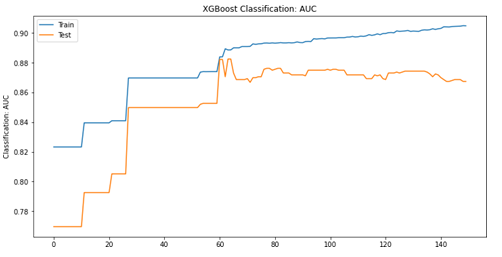
XGB: Classification score.
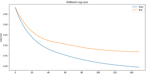
XGB: loss function. Figure 4: Evaluation performance for XGB model.
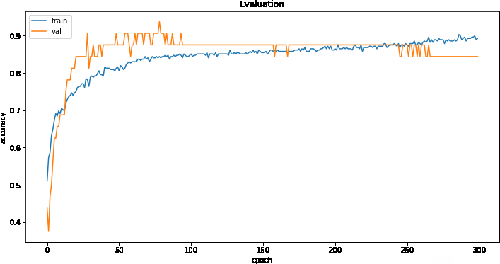
DNN: Accuracy score.
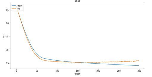
DNN: loss function. Figure 5: Evaluation performance for DNN model.
Experimental Results
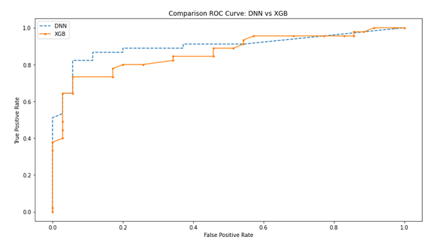
The two methods implemented on the available data, compared to the parameters described in the tables 1, 2 did not produce results so discrepant: the performances are quite similar and each of the two models responded significantly to the predictive task defined. As for the training and construction phase of the two models in comparison, the DNN model reports on the train and validation data set, respectively, an accuracy of 0.90 and 0.83, while the XGB respectively of 0.83 and 0.78: the most the predictive capacity of the models in the test phase on 10% of the data sampled from the initial validation set is significant: for each model, DNN and XGB, the accuracies are 0.93 and 0.80 respectively. The most interesting statistics, however, concern the two metrics of precision and recall, which respectively measure the fraction of cases correctly classified for a given class (i.e., Target = BC) on the total number of times that the model predict them, and is a good indication on the actual number of false positives, which in a context such as that of cancer research is certainly a very important element. Recall, on the other hand, is the fraction between the correct predictions for a class on the total of cases in which it actually occurs, and is also defined as the sensitivity of the model in recognizing false positives. The results obtained from the models for precision and recall on the test data, for the DNN and the XGB respectively are (0.93; 0.95) and (0.73; 0.89). From these two metrics we can calculate the F1-Score which is a harmonic average of precision and recall, in order to have an estimate of the best performance between the two, respectively for DNN and XGB the score is 0.94 and 0.80. In figure 6 it is possible to observe the comparison of the rate of false positives and true positives for the two models through the graph of the ROC curve (Receiver operating characteristic); it is observable that the performance of the DNN classifier is clearly superior to that of the XGB (Figure 6).
The figure 4 shows the performances obtained on the XGB model: it is possible to notice how with respect to the DNN model in figure 5, even if the data are in tabular format and despite optimization and hypertuning, the XGB metrics are lower. What previously observed on precision, recall and F1-Score is highlighted, for each class of the target variable, in the table 3, from which it is possible to deduce the significant differences between the two proposed methods. With a statistical approach based on the calculation of confidence intervals at a level of 95%, using the quantile of the Gaussian distribution, it is possible perform the analysis of the classification error for the two compared models: the classification error expressed in percentage terms, of the XGB is included in the interval [0.11;0.28] while for DNN [0.025 ;0.15]. It is possible to observe how the range of possible classification errors committed by the two models is much higher in the XGBoost than in the DNN, four times for the lower extreme and almost twice for the upper extreme of the confidence interval (Table 3).
| DNN | precision | recall | f1-score | support |
|---|---|---|---|---|
| BC | 0.94 | 0.92 | 0.93 | 36 |
| No-BC | 0.93 | 0.95 | 0.94 | 44 |
| accuracy | 0.94 | 80 | ||
| macro avg | 0.94 | 0.94 | 0.94 | 80 |
| weighted avg | 0.94 | 0.94 | 0.94 | 80 |
| XGB | precision | recall | f1-score | support |
| BC | 0.89 | 0.72 | 0.79 | 43 |
| No-BC | 0.73 | 0.89 | 0.8 | 37 |
| accuracy | 0.8 | 80 | ||
| macro avg | 0.81 | 0.81 | 0.8 | 80 |
| weighted avg | 0.82 | 0.8 | 0.8 | 80 |
Table 3: Evaluation report on test set: DNN vs XGB.
Final Remarks
The comparison between these two well known methods has produced encouraging and quite good results summarized as follows: the accuracy of the DNN equal to 0.90 on the train set and 0.83 on the validation set while the XGBoost respectively 0.83 and 0.78; higher performances obtained by the DNN also in terms of precision recall, for precision the DNN has a score higher than 25% and for recall of 6%. The F1-Score as a score for the DNN also results 17.5% higher than the XGBoost; the random intervals that contain the value of the classification error also in this case is better in the DNN, as well as the values obtained from the analysis of the ROC curve, with scores AUC of 0.93 and 0.86 respectively for DNN and XGBoost respectively.
Conclusions
The problem of breast cancer like other types of cancer, and their study remains a topic of fundamental importance for the development of effective treatments, artificial intelligence techniques are bringing countless scientific contributions: diagnoses performed by systems that use artificial intelligence are faster and more precise than those performed by the human operator [40], although still with some limitation. One of the main elements that characterize machine learning and AI more generally are data: the quantity and quality of data available provides the input with which the model, or the system, learns the patterns, and the heart of learning, or how the ”machine” thinks is all in a cost function, o loss function that through the data (examples) is able to recognize structures and patterns. Therefore what determines sure good output is what comes given to the algorithm or model as input. This work focuses on the type of data that can be considered for the purposes of an AI system in use in support systems to clinical decisions. The evolution of deep learning has made it possible to work on the images and data considered by means of the computing power available more traditional such as tabular ones, useful for teaching machine learning systems. Starting from the available data collected through a questionnaire, with a form of response or binary or multiclass, two methods were compared: the first is an ensemble model, the XGBoost which, due to its reputation, solves complex problems very accurately applying it to tabular data, the second is a neural network (DNN) which is notoriously used on unstructured data such as images and videos. The result obtained instead contradicts the hypothesis according to which a tool such as the DNN can be too complicated for such simple data, therefore the evidence of the work is not to reach a benchmark with the models in terms of precision, recall or accuracy, but to provide evidence on the possibility of using tools in any case of deep learning on tabular data. Last but not least, however, the case analyzed on real data coming from a questionnaire administered to an Indonesian female population remains of strong interest, firstly because it deals with real data on a real and complex problem, secondly because at the state of the art these problems, with these data are treated from a statistical point of view with case-control studies, therefore using these data, testing other non-statistical and non- parametric approaches, provides additional tools that I can contribute to the development of new methods, precise, accurate and useful for studying phenomena of interest such as the one object of the following work. This work could give rise to new ideas and interesting insights that involve the use of deel learning to other types of data; the case study it can represent a starting point and possibly be studied with other approaches and different observation possibilities.
References
-
Wang Y, Yang F, Zhang J (2021) Application of artificial intelligence based on deep learning in breast cancer screening and imaging diagnosis. Neural Comput and Applic 33: 9637-9647.
-
Chen H, Liu J, Wen QM (2021) CytoBrain: Cervical Cancer Screening System Based on Deep Learning Technology. J Comput Sci Technol 36(2): 347-360.
-
Becker AS, Mueller M, Stoffel E, Marcon M, Ghafoor S, et al. (2018) Classification of breast cancer in ultrasound imaging using a generic deep learning analysis software: a pilot study. Br J Radiol 91(1083): 20170576.
-
Ji Y, Li H, Edwards AV (2019) Independent validation of machine learning in diagnosing breast Cancer on magnetic resonance imaging within a single institution. Cancer Imaging 19(1): 64.
-
Antonelli M, Johnston EW, Dikaios N (2019) Machine learning classifiers can predict Gleason pattern 4 prostate cancer with greater accuracy than experienced radiologists. Eur Radiol 29: 4754-4764.
-
Zhang JK, He Y, Sobh N, Popescu G (2020) Label-free colorectal cancer screening using deep learning and spatial light interference microscopy (SLIM). APL Photonics 5.
-
Zhang H, Hu D, Duan H (2021) A novel deep learning approach to extract Chinese clinical entities for lung cancer screening and staging. BMC Med Inform Decis Mak 21: 214.
-
Li Q, Yang H, Wang P (2022) XGBoost-based and tumor- immune characterized gene signature for the prediction of metastatic status in breast cancer. J Transl Med 20: 177.
-
Yu Liew X, Hameed N, Clos J (2021) An investigation of XGBoost-based algorithm for breast cancer classification. Machine Learning with Applications 6.
-
Sugiharti E (2021) Convolutional neural Network- XGBoost for accuracy enhancement of breast cancer detection. Journal of Physics: Conference Series 1918.
-
Kabiraj S (2020) Breast Cancer Risk Prediction using XGBoost and Random Forest Algorithm, 2020 11th International Conference on Computing, Communication and Networking Technologies (ICCCNT) pp: 1-4.
-
Yulin Z, Tong F, Shudong W, Ruyi D, Jialiang Y, et al. (2020) A Novel XGBoost Method to Identify Cancer Tissue of Origin Based on Copy Number Variations. Frontiers in Genetics 11: 585029.
-
Nindrea R, Usman E, Katar Y, Darma I, Ricvan Dana N, et al. (2021) Dataset of Indonesian women reproductive, high-fat diet and body mass index risk factors for breast cancer. Data In Brief 36: 107107.
-
Shayan S (2018) Deep generative breast cancer screening and diagnosis. International Conference on Medical Image Computing and Computer-Assisted Intervention. Springer, Cham.
-
Franciszek B (2021) Radiomics and artificial intelligence in lung cancer screening. Translational lung cancer research 10(2): 1186-1199.
-
Hiba C, Zouaki H, Alheyane O (2018) Deep convolutional neural networks for breast cancer screening. Computer methods and programs in biomedicine 157: 19-30.
-
Causey Jason L (2019) Lung cancer screening with low- dose CT scans using a deep learning approach. arXiv preprint 1906.00240.
-
Huanhuan L (2021) A deep learning model integrating mammography and clinical factors facilitates the malignancy prediction of BI-RADS 4 microcalcifications in breast cancer screening. European Radiology 31(8): 5902-5912.
-
Geras Krzysztof J (2017) High-resolution breast cancer screening with multi-view deep convolutional neural networks. arXiv preprint 1703.07047.
-
Nan W (2020) Improving the ability of deep neural networks to use information from multiple views in breast cancer screening. Medical Imaging with Deep Learning.
-
Hunter P, Monahan C (2019) Genetic deep learning for lung cancer screening. arXiv preprint 1907.11849.
-
Socher R, Perelygin A, Wu J, Chuang J, Manning CD, et al. (2013) Recursive Deep Models for Semantic Compositionality Over a Sentiment Treebank. In: Proceedings of the 2013 Conference on Empirical Methods in Natural Language Processing, Seattle, Washington, USA, Association for Computational Linguistics pp: 1631–1642.
-
Socher R, Lin CC, Manning C, Ng AY (2011) Parsing natural scenes and natural language with recursive neural networks. In International Conference on Machine Learning. Omnipress pp: 129-136.
-
Mozetic I, Grcar M, Smailovic J (2016) Multilingual Twitter sentiment classification: The role of human annotators. arxiv: 1602.07563.
-
Wehrmann J, Becker W, Cagnini H, Barros RC (2017) A character-based convolutional neural network for language-agnostic Twitter sentiment analysis. In International Joint Conference on Neural Networks. IEEE pp: 2384-2391.
-
Neumann M, Thang V (2017) Attentive convolutional neural network based speech emotion recognition: A study on the impact of input features, signal length, and acted speech. CoRR arxiv: 1706.00612.
-
Zhao Y, Jin X, Hu X (2017) Recurrent convolutional neural networks for speech processing. In IEEE International Conference on Acoustics, Speech and Signal Processing. IEEE SigPort pp: 5300-5304.
-
Pascual S, Bonafonte A, Serr`a J (2017) SEGAN: Speech enhancement generative adversarial network. CoRR abs/1703.09452.
-
Krizhevsky A, Sutskever I, Hinton G (2012) ImageNet classification with deep convolutional neural networks. In: Advances in Neural Information Processing Systems 25. Pereira F, Burges CJC, et al. (Eds.). Curran Associates pp: 1097-1105.
-
Simonyan K, Zisserman A (2014) Very deep convolutional networks for large-scale image recognition. CoRR abs/1409.1556.
-
Girshick R, Donahue J, Darrell T, Malik J (2014) Rich feature hierarchies for accurate object detection and semantic segmentation. In IEEE Conference on Computer Vision and Pattern Recognition. IEEE pp: 580-587.
-
Karpathy A, Toderici G, Shetty S, Leung T, Sukthankar R, et al. (2014) Large scale video classification with convolutional neural networks. In IEEE Conference on Computer Vision and Patter.
-
Redmon J, Divvala S, Girshick S, Farhadi A (2016) You only look once: Unified, real-time object detection. In IEEE Conference on Computer Vision and Pattern Recognition. IEEE Computer Society pp: 779-788.
-
Hong S, Kim K (2010) An integrated GPU power and performance model. In The 37th International Symposium on Computer Architecture 38: 280-289.
-
Vasilache N, Johnson J, Mathieu M, Chintala S, Piantino S, et al. (2014) Fast convolutional nets with fbfft: A GPU performance evaluation.
-
Yadan O, Adams K, Taigman Y, Ranzato MA (2013) Multi- GPU training of ConvNets.
-
Kang X, Song B, Sun F (2019) A Deep Similarity Metric Method Based on Incomplete Data for Traffic Anomaly Detection in IoT. Applied Sciences 9(1): 135.
-
Srinivasan S (2021) Industry 4.0 Interoperability, Analytics, Security, and Case Studies.
-
Mashfiqur RSK (2019) Nonintrusive reduced order modeling framework for quasigeostrophic turbulence. Physical Review.
-
Tran KA, Kondrashova O, Bradley A, Williams ED, Pearson JV, et al. (2021) Deep learning in cancer diagnosis, prognosis and treatment selection. Genome Med 13(1): 152.
- Capacity Constraints in Pediatric Inpatient Psychiatric Care: A Cross-Sectional Analysis of Bed Availability and Geographic Access in North Carolina
- Why Healthcare Analytics Still Optimizes the Wrong Things
- Coding, Coverage, and Care: The Infrastructure of Transgender Health Inequities
- The Effect of Classroom Attendance on Academic Achievement of Management and Leadership Discipline of Nursing Students at Instituto Superior Cristal and Universidade de Dili, Timor-Leste, 2024: A Case Study
- The Role of Social Bonds in Facilitating Shared Investments and Resource Allocation: Addressing the “Wrong Pocket Problem” in Public Health and Healthcare
- Social-Cultural Factors Contributing to Antimicrobial Resistance in Livestock Farmers and Community Households in Kayonza District, Rwanda