Study the Structure of Phase Space in the Frame Work of Planar Circular Restricted Three-Body Problem

The Equations of Motion

Consider the more massive primary of mass is m1 and m2 is the mass of the smaller primary. These two masses have circular orbits about their common center of mass in a plane under the influence of their mutual gravitational attraction. A third body (attracted by the previous two but not influencing their motion) moves in the plane of primaries. To obtain the equations of motion for the third body, we choose XY as the sidereal frame and xy as the synodic frame. Let the co- ordinates of m1, m2 and m in the sidereal frame be (X1, Y1), (X2, Y2) and (X, Y), respectively, and that in the synodic frame be (x1, y1), (x2, y2) and (x, y), respectively as shown in Figure 1. To non-dimensionalise the problem, take unit of mass the total of the masses of M1 and M2, unit of length the distance between the primaries. These units force a gravitational constant G = 1. The only parameter in the system is the mass parameter μ.

Click to enlarge

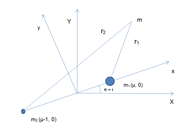
The transformation from synodic system (x, y) to sidereal system (X, Y) is given by cos sin sin cos X x t y t Y x t y t = − = + (7) In the Sidereal Frame:

2 2 1 KineticEnergy 2 T X Y   = +   (8)

( )

1 PotentialEnergy V r r µ µ   − = − −    

( ) (9)

1 2 where 𝑟1and 𝑟2 are the magnitudes of the position of the third body from the more massive primary and smaller primary, respectively.

The Lagrangian of the system is given as

• Lagrangian (L) = kinetic energy – potential energy
• Lagrangian (L) = T-V

1 1 2 X Y r r µ µ   −   = + − −      

2 2 (10)

1 2 Using equation (1), we get cos sin sin cos      

X x t x t y t y t

= − − − (11) sin cos cos sin Y x t x t y t y t

= + + − ( ) ( ) 2 2 2 2 X Y x y y x + = − +     (12)

Equation (4) now take the form ( ) ( ) ( ) 2 2

1 1 2 Langrangian L x y y x r r µ µ   −   = − + + −         (13)

1 2 where ( ) 2 2 2 1_r_ x y µ = − + (14)

( ) 2 2 2 2 1 r x y µ = + − + (15)

Differentiating 𝑟1 and 𝑟2 with respect to x and y, we get r x x r

µ ∂ − = ∂

1 (16)

1 r y y r ∂ = ∂

1

1

1 r x x r µ ∂ + − = ∂

0 d L L dt x x ∂ ∂  − =   ∂ ∂    (18)

0 d L L dt y y   ∂ ∂ − =   ∂ ∂    (19)

where L x y x ∂ = − ∂  

L y x y ∂ = + ∂  

( )( ) ( )

1 1 x x L y x x r r

µ µ µ µ − − + − ∂ = + − − ∂ 

3 3 1 2 ( )

1 y L y x y x r r

µ µ − ∂ = −+ − − ∂ 

3 3 1 2 Lagrange equation corresponding to equation (18) is [ ] ( )( ) ( )

1 1 0 x x d x y y x dt r r

µ µ µ µ − − + −   − − + − − =      

3 3 1 2 ( )( ) ( )

1 1 2 x x x y x r r

µ µ µ µ − − + −   − = − −       (20)

3 3 1 2 Let

1 1 2 x y r r µ µ   − Ω= + + +    

( ) 2 2 (21)

1 2 Equation (14) can be written as

2 x y n ∂Ω − = ∂   (22)

Lagrange equation corresponding to equation (19) is [ ] ( )

1 0 y d y y x x y dt r r

µ µ −   + + −+ − − =      

3 3 1 2 ( )

1 2 y y y x y r r

µ µ −   + = − −      

3 3 1 2

2 y x y ∂Ω + = ∂   (23)

Jacobi Integral Multiplying equation (16) by x and equation (17) by y, we get

2 xx yx x x ∂Ω − = ∂    (24)

2 yy xy y y ∂Ω − = ∂    (25)

Adding equations (18) and (19), we get x y xx yy t x t y ∂∂Ω ∂∂Ω + = + ∂ ∂ ∂ ∂   (26) Integrating equation (20), we get

2 2 1 1 1 2 2 x y C + = Ω+  

2 2 2 x y C + = Ω+   (27)

This is Jacobian integral. It will represent all possible motion for different values of Jacobi constant C.

Poincare Surface of Sections for Different Systems

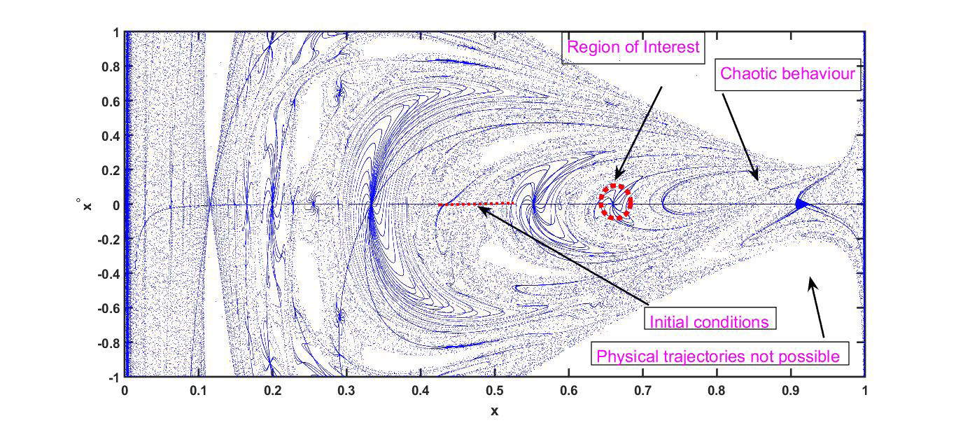
The PSS method is a simple, yet effective technique that can display the qualitative nature of a dynamical system in a single diagram. A surface of section is found by viewing the trajectory in a stroboscopic manner. A great number of trajectories are to be computed for this technique [2]. In this technique, the equations of motion (Eqn 22) and (Eqn 23) in chapter 1 were integrated using fourth-order Runge- Kutta-Gill method with integration step size ∆t of 0.0005. The initial conditions were selected along the x-axis and the magnitude of the velocity vector was determined from its functional dependence on the Jacobi constant. The surface of section technique is good at determining the regular or chaotic nature of the trajectory. If there are smooth, well defined islands, then the trajectory is likely to be regular and the islands correspond to oscillation around a periodic orbit. The largest of the quasi-periodic orbits corresponds to the maximum amplitude of oscillation around the periodic one. The regular regions of a PSS are defined by a periodic orbit involved by quasi-periodic orbits and are interpreted as regions of stability in the sense that outside them the motion is certainly unstable and inside them the motion is in general regular. The maximum amplitude of oscillation is used as a parameter to measure the degree of stability of a periodic orbit with respect to the region around it in the phase space. Any fuzzy distribution of points in the surface of section implies that the trajectory is chaotic and within the mostly-chaotic regions, there are small regions of regular behavior, such as the region of interest indicated by the red circle as shown in Figure 2.1. Additionally, note that certain areas of the map display appear completely blank. No map returns exist in these areas because physical trajectories are not possible in these regions of the phase space.

Click to enlarge

To study the dependence of Jacobi constant and mass ratio for different systems on the stability regions, PSS at C = 2.9 and 3.0 are considered. Figures 2.2-2.9 shows the nature of phase plane corresponding to the decreasing order of mass ratio from the Sun- Jupiter to the Sun- Mercury system. The PSS of Sun-Jupiter system with mass ratio 0.0009537284, being the highest among the systems is generated for Jacobi constant C = 2.9 shown in Figure 2.2. In case of the fuzzy distribution of points, the region x = 0.55 to 0.65 is less for C = 2.9 and is more for C = 3.0. The stability region from x = 0.6 and 0.75 corresponding to the Jacobi constant C = 2.9 contain a number of invariant curves and with increase in the value of C from 2.9 to 3.0, this stability region disappeared. The stability region at x = 0.27 for C = 2.9 correspond to the periodic orbit around the Sun and as C increases from 2.9 to 3.0, this stability region moves towards the Jupiter.

The phase planes corresponding to the Sun-Uranus system given in Figures 2.2 & 2.3 show the number of invariant curves is less in each stability region. In case of the fuzzy distribution of points, it is more in the region from x = 0.0 to x = 0.20 for C = 2.9. The phase plots show that the stability region moves towards the right as C increases from 2.9 to 3.0. Chains of several resonant islands are identified after x = 0.75 for C = 2.9 and as C increases to 3.0, the size of

PSS for the Sun-Jupiter System

Click to enlarge

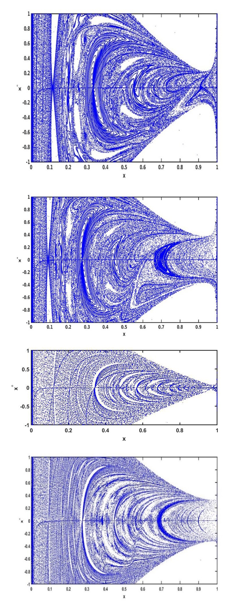
this resonant islands decreased.

The phase planes corresponding to the Jupiter-Io system are given in Figures 2.6 & 2.7. The phase plots show a number of islands with different size and shape and having comparatively small amplitudes with respect to the Sun- Jupiter system for Jacobi constant C = 2.9. In case of the fuzzy distribution of points, it is less in the region from x = 0.3 to x = 0.70 for C = 2.9 and is more for C = 3.0. Empty region is seen from x = 0.7 onwards, when C is increased from 2.9 to 3.0.

Figure 2.8 gives the phase plane corresponding to the Sun- Mercury system for C = 2.9. Fuzzy distribution of points is more in the region from x = 0.0 to x = 0.6 and number of islands are less in the phase plane. As C increases to 3.0, fuzzy distribution of points increased after x = 0.7. The stability regions after x = 0.25 move towards the Jupiter as C increases from 2.9 to 3.0.

PSS for the Jupiter-Io System

Click to enlarge

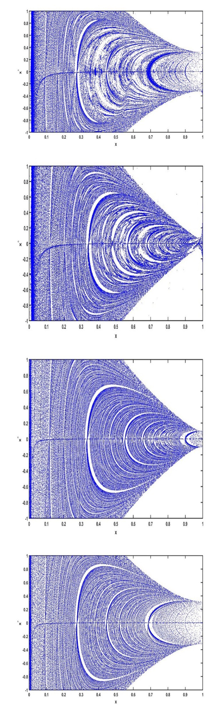
PSS for the Sun-Mercury System

References

-
Poincare H (1892) The New Methods of Celestial Mechanics. In: Goroff D (Ed.), History of Modern Physics and Astronomy, France 1: 82.
Murray CD, Dermot SF (1999) Solar System Dynamics. Cambridge University Press.
Boucher K (2004) The restricted three-body problem. Phys, Hamiltonian Dynamics 349: 1-27.
Kolmen E, Kasdin NJ, Gurfil P (2007) Quasi-periodic orbits of the restricted three-body problem made easy. New trends in astrodynamics and applications. American Inst of Physics, USA 886: 68-77.
Beevi SA, Sharma RK (2011) Analysis of periodic orbits in the Saturn–Titan system using the method of Poincare section surfaces. Astrophysics and Space Science 333: 37-48.
Nishanth P, Sharma RK (2017) Interior Resonance Periodic Orbits in Photogravitational Restricted Three- body Problem. Advances in Astrophysics 2(1): 263-272.
Kumar P, Sharma RK (2019) On merging of resonant periodic orbits 4:3; 3:2 and 2:1 in Sun-Jupiter photo gravitational restricted three-body problem. International Journal of Advanced Astronomy 7(1): 17- 24.
Kumar P, Guptha ESD, Mourya MKJ, Pranav SV (2023) Evolution of Periodic Orbits in the Sun-Jupiter and Sun- Earth Systems. Indian journal of science and technology 16(10): 717-726.
Pathak N, Thomas VO, Abouelmagd I (2019) The perturbed photogravitational restricted three body problem: Analysis of resonant periodic orbits. Discrete and continuous dynamical systems series 12(4-5): 849- 875.
- Early Universe: Hadronic Crystals Coherent Micro Gravitational Wave Emitters PHYSICS Part II
- The Solar System Constraint Maze: A Scientific Dead-End Revealing the Interuniversal Machine
- Assessment of Radiofrequency Radiation from 2G and 3G Mobile Phone Handsets
- Early Universe Magneto-Gravitational Coupling Genesis Physics: Part I
- Falsifiability of the Classical Law of Gravitation and Unveiling the Time-temperature Entanglement of the Universe
- Origin of Ancient Civilisations The Southern Hemisphere’ Scenario