Improvement of Calculations for Turbulent Premixed Flame Characteristics Determination using PDF Monte Carlo Simulation
This study aims at simulating turbulent premixed flame in a constant-pressure vessel (P = 1 atm) where the turbulence is supposed to be homogeneous and isotropic. The mixture of gas is composed by iso-octane-air. The realized CFD were based on Lagrange approach in Monte Carlo simulations. We focused on calculations of; flame radii RF, the flame propagation velocity St, flame-brush thickness ï¤t and flammability limit. During the study, influencing crucial parameters such as, the equivalence ratio ï¦ and the turbulence intensity u’ were considered. Results show that the equivalence ratio enhances the flame propagation when passing from lean to stoichiometric flames. Also, the turbulence intensity yields a notable growth for the flame characteristics mentioned above. Moreover, we noticed that the flammability limit is strongly depending of the turbulence intensity and the equivalence ratio. More precisely, we remarked that the minimum ignition energy (MIE) was situated quite smaller than the stoichiometric condition. But, it increased with the turbulence intensity.
Introduction
Although the trend nowadays is towards more and more renewable energy such as; solar energy (thermal and/or photovoltaic), wind energy, geothermal energy and especially biomass [1, 2, 3, 4], the fossil energies used in combustion in various installations still retain their importance [5, 6, 7, 8]. However, although turbulent premixed flames were well studied [9, 10, 11], and for more than 50 years ago, we think that many aspects of the problem remain misunderstood. Indeed, significant practical problems still remain not resolved in spark-ignition engines, explosions and stationary power gas turbine. In this context many works in literature are dealing with spherical expanding laminar/turbulent flames. Shu, et al. [12] developed an experimental study of laminar ammonia-methane-air premixed flames based on expanding spherical flames in a constant pressure chamber. They focused on the laminar flame speed, the Markstein lengths and the flammability limits. They found that the laminar flame speed correlated with the methane volume fraction. Also, when increasing methane content in the fuel mixture, upper and lower flammability equivalence ratio limits were boarded. Moreover, Bradley, et al. [13] focused on extending the measurements of turbulent burning velocity over a wide range of fuels and pressures using schlieren high speed photography to define the rate of burning and the smoothed area of the flame front. They obtained correlations of turbulent burning velocity normalised by the effective rms µ µ for a certain range of Karlovitz stretch factor (K) and ' t k different negative strain rate Markstein numbers. They concluded that ' t µ µ increased when K decreased. In addition, t authors identified different burning regimes from mixed turbulence/laminar instability at low K values to that corresponding to high K values for which µ µ is reduced due ' t t to localised flame extinctions. Nie, et al. [14] studied the flame height and the flame brush thickness of lean turbulent premixed Bunsen methane/air and propane/air flames. They observed that under fuel-lean conditions the Bunsen flame height and the centreline flame brush thickness decrease when increasing the equivalence ratio. However, the turbulence intensity plays a marginal role on these two parameters. Many other results reported in literature showed that the flame propagation velocity St is always increased by the root mean square (r. m .s.) u’ [15, 16, 17]. Indeed, the pioneers Damköhler [18] and Shchelkin [19] in this domain attributed the St Increase, under u’ effect, to the local flame surface area growth due to small-scale eddies. Also, in a previous paper, it was found that the flame burning velocity ratio St/SL followed a linear tendency according to the Damköhler model with n = 1 [20]. Concerning the flame-brush thickness δt, it is well known that this characteristic is quite affected by the equivalence ratio, but, more seriously by the turbulence intensity [9, 11, 21]. It is well known that the flame front propagation is governed by the success of the flame kernel initiation. The latter flame stage is seriously affected by flammability limits. Indeed, physical phenomena such as the flame stretch and the preferential diffusion controlled by turbulence, which influence seriously the flame burning velocity, are fundamental for understanding the flame extinction [22]. Hence, regarding what was reported in literature, the main object consists at knowing the behaviour of the flame, its propagation, the flame laminar speed, the flame burning velocity and the so-called flame-brush thickness constitute crucial data for more apprehending this type of combustion [23, 24, 25].
The investigated simulation in this paper is based on Monte Carlo method. This method is powerful when simulating the transport equations of joint probability density functions (pdf’s) in turbulent reactive. The whole space is the product of phases and thermochemical variables [26, 27]. Indeed, it was proven that the fluid particle, the probabilistic particle and the stochastic particle present almost the same trajectories in real, conditional and stochastic spaces respectively [28]. Hence, the principal objective in this work was to simulate turbulent premixed flame of iso-octane/ air using Monte Carlo method in a lagrangian approach. For this purpose we tried to extend the simulation time as long as possible. As it is explained below this method requires multi-level modelling; on the correlated velocity field, on the turbulent diffusion and on the chemical kinetics of reaction and reaction rate. The parameters affecting the flame development are the equivalence ratio and the turbulence intensity (rms). Appropriate treatments of the temperature field inside the combustion chamber permit the access to determine the up-mentioned flame characteristics.
Formulation and Operating Conditions
The governing equations for this problem are; the mass conservation equation written in spherical coordinates (Equation 1) (because of the spherical symmetry problem), the joint PDF transport equation (Equation 2) and the perfect gas equation (Equation 3).
( ) 2 2 1 0 r r t r r ρ ρ µ ∂ ∂ + = ∂ ∂ (1)
( ) ( ) ( ) ( ) ( ) ( ) , , , , , | , , u i u i u i i f f A f t x ϕ ϕ ϕ ρ ψ ν ψ ρ ψ ν ν ψ ν ψ ν ψ ν ∂ ∂ ∂ + = − ∂ ∂ ∂ ( ) , | , , uf α ϕ α θ ν ψ ν ψ ϕ ∂ − ∂ (2) with respectively:
∂ = + ∂
τ ρ ρ
1 i j i i j A F x ∂ = + + ∂
α J S x
. 1 k α α α θ ρ ω ρ j rT P M ρ = (3)
ρ is the density, ur is the radial velocity vector. In equation (4) Ø is the sample space variable corresponding to Ö and V is the sample space vector corresponding tou . f u Ö , is the joint PDF of velocities and scalars. The terms Ai andèá , which are characterized by stochastic processes, contain respectively the following physical terms: ôij is the viscous stress tensor, F i is the external force per volume unity, P is .
á kJ the diffusive fluxes, á ù the pressure, the reaction rate and finally á S the source term which provokes ignition. In equation (3), T is the temperature and M is the mean molecular weight of mixture.
The turbulence is supposed homogeneous and isotropic described by K-ε frozen model [29, 30]. However, we don’t take into account the interaction between flame and walls, and for overcoming this we suppose that the vessel is big enough and the kernel flame is ignited in the middle so that it can be developed far from the side walls. Chemistry
is simplified to a one stage global reaction and the reaction rate is calculated using Westbrook and Dryer formula [31]. Also, radiative transfers are not considered. Ignition energy comparable to that given by a spark in real case is deposited in a reduced zone characterized by a certain radius Rign, and during a certain time ∆tign. The spark ignition is selected to decrease linearly versus the time according to experimental observations and to decrease as a parabolic function like the variation of the loss of heat between the electrodes. Then, the whole energy produced by ignition is obtained by making the sum of the variations of enthalpy on all the elementary shells located inside the ignition radius. Before each run, we have fixed the kinetic energy of turbulence K, the dissipation rate of turbulence ε, the equivalence ratio Φ, the grid size dr, the time increment dt, the ignition radius Rign, the ignition time ∆tign, a constant characterizing the mixing frequency and the energy activation Ea. The turbulence intensity u’, the turbulent scale length Lt and the turbulent time scale τt are calculated in function of K and ε according to the K-ε frozen model:
3/2 0.16 t k L ε = (4)
å 3.0 = ô k t (5)
0.16 and 0.3 are two constants chosen on experimental considerations.
The flame propagation velocity is calculated by differentiating the flame radius as function of the time:
dR S dt = (6)
F t
The flame-brush thickness is evaluated using the following expression:
1 δ = (7) t dC max( )
dx In the last expression C is the progress variable, which is equal to zero in the fresh gas and, it is equal to 1.0 in the burned gas.
Mote Carlo Method
Because of the spherical symmetry of the problem, we carried out the numerical simulation in 1-D spherical case (a long an axis [O, R]). This domain should be divided into N cells. Initially, each cell should contain Ni particles. The pressure, supposed constant, is equal to 105 Pa. The micro-scale mixing imbedded in èá (in the second right hand side of (Equation 2)) occurs in a closed form and has to be modelled. The modified Curl micro-scale model was chosen based on coalescence–dispersion of particles [32]. Coalescence –dispersion models are also known as particle- interaction model in which mixing takes place by pairs: two particles Pi and Pj selected randomly from the ensemble of Nc particles in a given cell, mix with a certain probability Pm during a time step Δt. After mixing, the particles will have new scalar values, equal to the mean of their values before the mixing stage. Moreover, Monte Carlo particles are able to roam the domain randomly thanks to the expansion velocity and to the turbulent diffusion. The type of PDF that we use in this work, is the evolution PDF (transported PDF), called Pope’s method [28, 33, 34]. This method uses Monte Carlo particles solver, and the form of the PDF may freely evolve. Contrary to presumed PDFs, there is no preset shape in our case. The Monte Carlo method represents the PDF with an ensemble of “stochastic elements” distributed throughout the flow field, from which the moments of interest may be calculated. Particularly, in Lagrange approach, the elements (particles) are free to roam the physical domain as dictated by a stochastic hydrodynamic field. Moreover, the composition of elements changes only due to mixing and reaction. The particles enclosed in every cell are moved according to the local time step determined by the minimum of the flow time scale and the mixing time scale. In this context, Raman, et al. [35] performed some numerical tests to determine the optimal global time step, the optimal space step, and to estimate the increase in computation load with the number of particles per cell and, consequently the number of particles in the whole domain. They concluded that the tracking time scales linearly with particles, size grid and global time step. It was for Raman, et al. [35] that for the propane-air a time step of 2.10-4s yields consistent results for both reacting and non-reacting cases. Concerning statistical error, it can be noticed that it evolves like N-1/2, according to the central limit theorem. So, for a large number of particles, the error tends to zero, but the computational load increases hyper linearly. This result was also mentioned by Pope [28]. It is to be highlighted that the stochastic particles move in the calculation domain thanks to types of speeds:
- Gas expansion mean velocity due to temperature gradient between burned gas and fresh gas.
- Turbulent diffusion correlated velocities, based on Box and Müller transformation [36].
Results and Discussions
Mesh Effect
First of all, we tested the grid mesh size effect on the flame formation and propagation. For this, we varied the grid size dr at the vicinity of the optimal value stated by Raman, et al. [35], whereas, all the other simulation parameters were constant. Figure 1 shows that the grid size has a quiet little effect on the flame kernel formation. Furthermore, for these values the flame kernel was born and propagated without any difficulty.
40x10 -3 u' = 1.68 m.s-1 φ = 1.0
30 RF (m)
20 ∆ r = 2.5 10-4 m ∆ r = 3.0 10-4 m
10 ∆ r = 3.5 10-4 m
0
12x10 -3 10 8 6 4 2 0 Time (s) Figure 1: Effect of the grid size on the flame growth.
Minimum Ignition Energy (MIE)
To test the influence of the ignition energy Ien on the flame we carried out different runs with different ignition energies. Figure 2 illustrates that Ien plays an important role either on the flame kernel birth or on the flame propagation. Indeed, on one hand, more Ien is bigger more the flame kernel is early formed. On the other hand, it can be noted that high the ignition energy is, high the acceleration of the flame propagation is. This result can be attributed to the increase of temperature (reaching 2800 K) in the ignition zone of Rign radius. However, in order to more apprehend the problem of ignition fail (flammability limit) it is capital to optimise the minimum ignition energy (MIE) provided by the spark during the ignition step [22]. Obviously this phenomenon is not suggested in SI engine, although it is well recommended in order to bring down the number of accidents in mines and in industry. However, the ignition success/fail is not depended only on MIE. Indeed, the MIE may correlate with the equivalence ratio and also with the turbulence intensity. Figure 3 shows the variation of MIE with the equivalence ratio Φ. This curve is similar to what was published in literature by Lewis and von Elbe [37]. MIE minimal founded in our case iso-octane/air flame is 0.4 mJ for Φ = 0.95 and rms u’ = 0.2 m/s. The value founded by Lewis and von Elbe for CH4/air laminar flame was 0.3 mJ for Φ = 0.9. The little difference can be attributed to the weak turbulence in our case. In the same context, Figure 4 shows the variation of MIE versus the equivalence ratio for different turbulence intensities u’. It can be noted that when increasing u’ MIE increases, but the equivalence ratio corresponding to MIE is always at the vicinity of 09-0.95. This shows that the turbulence plays a negative role on the flame kernel formation, and in many case the flame can’t resist to the wrinkling and stretching effects caused by turbulence, and leading to flame extinction [38, 39].
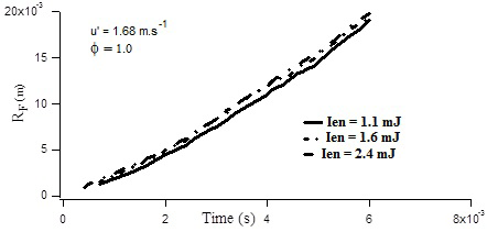
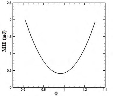
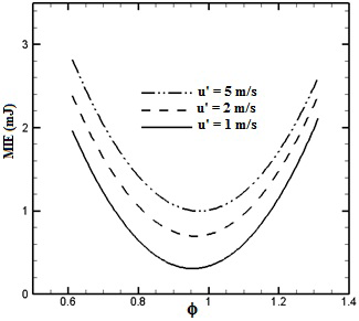
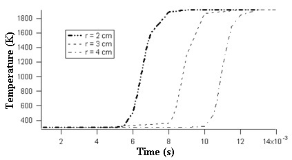
Figure 5: Evolution of the temperature as function of elapsed time for different radii from the ignition zone Figure 6 shows the variation of the flame radius versus elapsed time, for different equivalence ratios and for a given turbulence intensity. One observed that lean flames exhibited quite linear radius. However, when we go near the stoichiometric flames, radius becomes more and more parabolic. Hence, the flame is accelerated when reaching stoichiometric condition.
50x10 -3 φ = 0.85
40 u' = 1. m/s u' = 1.5 m/s u' = 1.68 m/s u' = 2. m/s u' = 2.5 m/s
30 RF(m)
20
10
12x10 -3 10 8 6 4 2 Time (s) Figure 7: Temporal evolution of the flame radius for different turbulence intensities.
Figure 7 shows the turbulence intensity effect on the flame radius evolution for a given equivalence ratio. One noticed that radii become more parabolic when increasing the turbulence intensity u’. This result could be attributed by a turbulent diffusion more efficient when the turbulence is more intense. Indeed, the micro-scale mixing becomes more efficient. Figure 8 illustrated a good agreement between our results and those obtained experimentally by Groff in similar conditions [40].
40 by Groff Monte Carlo simulation
30 RF(mm)
20
10
14 12 10 8 6 4 2 Time (ms) Figure 8: Flame radius evolution versus elapsed time. Comparison with [40].
Flame Propagation Velocity
Figure 9 shows the influence of the equivalence ratio on the flame propagation speed St. Lean flames (Φ = 0.7 and Φ = 0.8) this figure exhibit almost constant speed. However, when increase the equivalence ratio, the flame propagation velocity increases and tends to an asymptotic value in the case of a moderate turbulence (u’=1.2 m/s). In Figure 10 the effect of the turbulence intensity is tested for a given equivalence ratio. Even in the case of lean flame the increase of the flame propagation speed is notable. Furthermore, the growth of speed can reach un-controlled level with intense turbulence (no asymptotic tendency in this case). In Figure 11 we carried out comparisons with results found by Lipatnikov and Chomiak [41], and Bradley, et al. [42].
7 u' = 1.2 m.s -1
φ = 0.7
6 φ = 0.8 φ = 0.9 φ = 1.0
5 St ( m.s-1 )
12x10 -3 10 8 6 4 2 Time (s) Figure 9: Evolution of the flame propagation velocity versus elapsed time for different equivalence ratios.
All flames are spherical and developing in chambers where an homogeneous and isotropic turbulence occurs with an integral length scale Lt = 20 mm. The initial temperature of iso-octane-air mixture is equal to 358 K. The pressure is equal to 105 Pa. The equivalence ratio is equal to 0.8 and the turbulence intensity value is u’ = 2.36 m.s-1. We observe that curve obtained by Monte Carlo simulation is in a satisfactory agreement with both F.S.C. model [41] and experimental [42]. However, the agreement is better with Bradley, et al. [42] when the flame radius is ranging between 15 and 30 mm.
8 φ = 0.8 u' = 0.7 ms -1
u' = 1.1 ms -1
6 u' = 2.50 ms -1
St ( m.s-1 )
12x10 -3 10 8 6 4 2 0 Time (s) Figure 10: Evolution of the flame propagation velocity versus elapsed time for different turbulence intensities.
u' = 2.36 ms -1
8 φ = 1.0
6 St( m.s-1 )
experimental after Bradley et al. Calculations after Bradley et al. FSC model Monte Carlo simulation
50x10 -3 40 30 20 10 0 RF (m) Figure 11: Evolution of the flame propagation velocity versus its radius.
12 10 8 6 4 2 t/ τt Figure 12: Variation of the dimensionless flame-brush thickness versus the dimensionless time, for three turbulence intensities.
Figure 12 shows the evolution of dimensionless flame brush thickness versus dimensionless time. Simulations runs are conducted for different turbulence intensities and a fixed equivalence ratio near stoichiometric condition. One observed that δt/Lt increases up to an asymptotic value in each case. The asymptotic value increases with the rms u’. This result is in agreement with theoretical predictions because the main effect of turbulence on flame consists at increasing its surface density and thereby its propagation speed.
In Figure 13 are plotted the dimensionless flame brush thickness as function of the dimensionless time for different equivalence ratio and for a fixed turbulence intensity u’. As it is shown δt/Lt increases rapidly at the beginning and tends to an asymptotic value. Also, one noticed that this limit value increases when the equivalence ratio decreases in perfect predictions with the combustion regimes diagram. In addition, it is to be highlighted that this phenomenon appears only when the flame becomes developed enough (t/ τt > 2.0).
0.6 φ = 0.9 φ = 0.8 φ = 0.7
10 8 6 4 2 0 t/ τt Figure 13: Variation of the dimensionless flame-brush thickness versus the dimensionless time, for three equivalence ratios.
Conclusion
We carry out numerical simulation of premixed turbulent spherical flame using Monte Carlo method in lagrangian approach. Results show that for optimal space step of 2 10-4 m and optimal time step of 10-4s the calculation load is acceptable. Moreover, we remark that the MIE is situated closed the stoichiometric condition (Φ ≈ 0.95). The premixed flame characteristics such as, flame radius, flame propagation speed and flame brush thickness are strongly influenced by the turbulence intensity, but less by the equivalence ratio. The flame propagation speed is almost constant for lean flames but increases to an asymptotic value. But, in case of high intensity of turbulence the growth becomes uncontrollable. The same bending effect seen for the flame propagation speed is also observed with the flame brush thickness.
References
-
Zribi M, Lajili M, Escudero-Sanz FJ (2018) Hydrogen enriched syngas production via gasification of biofuels pellets/powders blended from olive mill solid wastes and pine sawdust under different water steam/nitrogen atmospheres. International Journal of Hydrogen Energy 44(22): 11280-11288.
-
Mami MA, Mätzing H, Gehrmann HJ, Stapf D, Bolduan R, et al. (2018) Investigation of olive mill solid wastes pellets combustion in a counter-current fixed bed reactor. Energies 11(8): 1-21.
-
Khlifi S, Lajili M, Tabet F, Boushaki T, Sarh B (2020) Investigation of combustion characteristics of briquettes prepared from olive mill solid waste blended with and without a natural binder in a fixed bed reactor. Biomass Conversion and Biorefinery 10(2): 535-544.
-
Heidenreich S, Foscolo PU (2015) New concepts in biomass gasification. Progress in Energy and Combustion Science 46: 72-95.
-
Sheykhi M, Chahartagni M, Pirooz AAS (2020) Investigation of effects of operating parameters of an internal combustion engine on the performance and fuel consumption of a CCHP system. Energy 211.
-
Giménez B, Melgar A, Horrillo A, Tinaut FV (2021) A correlation for turbulent combustion speed accounting for instabilities and expansion speed in a hydrogen- natural gas spark ignition engine. Combustion and Flame 223: 15-27.
-
Weber R, Gupta AK, Mochida S (2020) High temperature air combustion (HiTAC): How it all started for applications in industrial furnaces and future prospects. Applied Energy 278.
-
Agwu O, Runyon J, Goktepe B, Chong CT, Ng JH, Giles A, Valera-Mdina A (2020) Visualisation and performance evaluation of biodiesel/methane co-combustion in a swirl-stabilised gas turbine combustor. Fuel 277: 2-9.
-
Kwon S, Wu, MS, Driscoll JF, Faeth, GM (1992) Flame surface properties of premixed flames in isotropic turbulence: Measurements and numerical simulations. Combustion and Flame 88(2): 221-238.
-
Herweg, R, Ziegler, GF (1990) Flame Kernel Formation in a Spark-Ignition Engine. International Symposium COMODIA, Japan, pp: 173-178.
-
Bielert U, Klug M, Adomeit G (1996) Application of front tracking techniques to the turbulent combustion processes in a single stroke device. Combust Flame 106: 11-28.
-
Shu T, Xue Y, Zhou Z, Ren Z (2021) An experimental study of laminar ammonia/methane/air premixed flames using expanding spherical flames. Fuel 290: 1-10.
-
Bradley D, Lawes M, Liu K, Mansour MS (2013) Measurements and correlations of turbulent burning velocities over wide ranges of fuels and elevated pressures. Proceedings of the Combustion Institute 34(1): 1519-1526.
-
Nie Y, Wang J, Zhang W, Chang M, Zhang M, et al. (2019) Flame brush thickness of lean turbulent premixed Bunsen flame and the memory effect on its development. Fuel 242: 607-616.
-
Aldredge RC, Vaezi V, Ronney PD (1998) Premixed- flame propagation in turbulent Taylor-Couette flow. Combustion and Flame 115(3): 395-405.
-
Kido H, Kitagawa T, Nakashima K, Kato K (1989) An improved model of turbulent mass burning velocity. Memoirs of the Kyushu University, Faculty of Engineering 49(4): 229-247.
-
Gillespie L, Lawes M, Sheppard CGW and Woolley R (2000) Aspects of Laminar and turbulent Burning Velocity Relevant to SI Engines. SAE Technical Paper Series 109(3): 13-33.
-
Damköhler G (1940) Der Einfluss der turbulenz auf die flammengeschwindigkeit in gasgemischen. Z Electrochem 46(11): 601-626.
-
Shchelkin KI (1947) Combustion in turbulent flow. Zhournal Technicheskoi Fisiki 13:520-530.
-
Lajili M, Said R (2008) Study Of The Flame-Burning Velocity Ratio Using PDF Monte Carlo Model. Combustion Science and Technology 180(5): 785-795.
-
Lipatnikov AN, Chomiak J (2004) Turbulent Flame speed and thickness: Phenomenology, evaluation, and application in multi-dimensional simulations. Prog Energ Combust Sci 28(1): 1-74.
-
Kono M, Tsue M (2009) Flammability limits: Ignition of a Flammable Mixture and Limit Flame Extinction. In: Jarosinski J, Veyssiere B (Eds.), Combustion phenomena selected mechanisms of flame formation, propagation and extinction. 1st(Edn.), CRC Press, Taylor & francis group, New york, USA.
-
Kelly AP, Law CK (2009) Nonlinear effects in the extraction of laminar flame speeds from expanding spherical flames. Combustion and Flame 156(9): 1844- 1851.
-
Fruchard N, Borghi R (1997) Turbulent combustion modeling–ignition and initial period of propagation. Progress in Astronautics and Aeronautics 173: 221-233.
-
Karlin V, Sivashinsky G (2006) The rate of expansion of spherical flames. Combustion Theory and Modelling 10(4): 625-637.
-
Pope SB (1980) Monte Carlo Method for the PDF Equations of Turbulent Reactive Flow. Combustion Science and Technology 25(5-6): 159-174.
-
Mura A, Galzin F and Borghi R (2003) A unified PDF- Flamlet Model for Turbulent Premixed Combustion. Combustion Science and Technology 175(9): 1573-1609.
-
Pope SB (1985) PDF methods for turbulent reactive flows. Progress in Energy and Combustion Science 11(2): 119-192.
-
Gorji S, Seddighi M, Ariyarathe C, Vardy AE, O’Donoghue T, Pokrajac D, He S (2014) a comparative study of turbulence models in a transient channel flow. Computer & Fluids 89: 111-123.
-
Van der Laan MP, Andersen SJ (2018) The turbulence scales of a wind turbine wake: A revist of extended k-epsilon models. J Phys Conf Ser 1037(7): 1-10.
-
Westbrook CK, Dryer FL (1984) Chemical kinetic modeling of hydrocarbon combustion. Progress in Energy and Combustion Science 10(1): 1-57.
-
Ren Z, Pope SB (2004) An investigation of the performance of turbulent mixture models. Combustion and Flame 136(1-2): 208-216.
-
Pope SB (1994) Lagrangian PDF methods for turbulent flows. Annual Review of Fluid Mechanics 26: 23-63.
-
Haworth DC, Pope SB (1987) Monte Carlo solutions of a joint PDF equation for turbulent flows in general orthogonal coordinates. Journal of Computational Physics 72(2): 311-346.
-
Raman V, Fox RO, Harvey AD (2004) Hybrid finite- volume/transported PDF simulations of partially premixed methane-air flame. Combustion and Flame 136(3): 327-350.
-
Box GEP, Müller ME (1958) A note on the generation of Random Normal Deviates. Annals of Mathematical Statistics 29(2): 610-611.
-
Lewis B, Von Elbe G (1987) Combustion, Flames and Explosions of Gases. 3rd(Edn.), Academic Press, New York, USA.
-
Dunn MJ, Masri A R, Bilger R W, Barlow RS, Wang GS (2009) The compositional structure of highly turbulent piloted premixed flames issuing into a hot coflow. Proceeding of the Combustion Institute 32(2): 1779- 1786.
-
Dunn MJ, Masri A R, Bilger R W, Barlow R S (2010) Finite rate Chemistry Effects in Highly Sheared turbulent Premixed Flames. Flow Turbulence and Combustion 85: 621-648.
-
Groff EG (1982) The cellular nature of confined spherical propane-air flames. Combustion and Flame 48: 51-62.
-
Lipatanikov AN, Chomiac J (2004) Turbulent flame speed and thickness: Phenomenology, evaluation, and application in multi-dimensional simulations. Progress in Energy and Combustion Science 28(1): 1-74.
-
Bradley D, Lawes M, Sheppard CGW (1995) Study of turbulence and combustion interaction: measurements and predictions of the rate of turbulent burning. Report Leeds University.
- Nigeria’s Vulnerability in the Face of Global Energy Policy
- A Simulation Study of Investigation of Optimum Oil Production Performance by Applying Various Gas Injection Methods in Oil Reservoir
- Characterization of Permo-Triassic Reservoirs through Thermal Maturity Assessment of Westphalian Source Rocks in the Cheshire Basin
- Influence of Microwax on the Rheological and Thermal Behaviour of a Wax Crude Oil
- Real-Time Monitoring and Performance Optimization of Steam Injection in Heavy Oil Reservoirs Using Fiber Optic Sensing and Integrated Predictive Simulation Models
- Rapid On-Site Determination of the Total Petroleum Hydrocarbon Content of Soils by Handheld Fourier Transform Near-Infrared Spectroscopy: Development of a Global, Site- and Scanner- Independent Calibration Model