How Oil and Gas Companies can derive C-Factors in the API RP 14E Erosional Velocity Models for their ‘Clean Service’ Pipelines
In designing pipeline facilities for production and transportation of oil, hydrocarbon gases or non-hydrocarbon gases – CO2 and H2, consideration is given to pipeline integrity, flow assurance, operation and health/safety issues. Erosion-corrosion of the inner pipeline wall and/or high-pressure losses is of great concern. For many years now, many oil and gas field operators have adopted the America Petroleum Institute recommended practice 14E (API RP 14E) equation to estimate the erosional velocity. Unfortunately, the C-factor (which is an empirical constant) in the API RP 14E equation has been generalized to all field conditions. In addition, there is no concrete scientific evidence behind the basis of its formulation, and various values have been adopted based on field and laboratory experiences. In this work, we present how oil and gas companies could formulate safer erosional velocity models for their sand free or ‘clean service’ pipelines, based on the velocities calculated for the equilibrium flow rate (that is, the intersection of vertical lift performance (VLP) and inflow performance relationship (IPR)). The developed erosional velocity models can be applied, and compared with in-house correlations, for erosional velocity predictions.
Introduction
Erosion-corrosion is one of the primary contributing factors to pipeline failures and leaks; generally, the influencing variables are fluid related (flow velocity, corrosivity of liquid phase, flow regime, solid particle content), in addition to the pipe properties. Erosional velocity (that is, a velocity below which no erosion-corrosion is assumed to occur) greatly influences tubing sizing in the design stage; oversizing of tubing unnecessarily increases construction costs whilst underestimating the required size of tubular can lead to catastrophic erosion/corrosion failures [1]. To avoid erosion damage, the common oil industry practice for sizing process piping, flow lines, pipelines, and tubing is to limit the flow velocity to the maximum erosional velocity as given in Equation 1, the API RP 14E equation [2].
$$V_e = \frac{C}{\sqrt{\rho_m}}$$ (1)
where $V_e$ is fluid erosional velocity, ft/s; $C$ (100 for continuous service, 125 for intermittent service for both solid-free flowing fluid, and reduced value if solid particles are present) is an empirical constant; $\rho_m$ is gas/liquid mixture density at flowing pressure and temperature, lb/ft³ (API RP 1984). The fluid mixture density $\rho_m$ is calculated using Equation 2.
$$\rho_m = \frac{12409S_jP + 2.7RS_gP}{198.7P + RTZ}$$ (2)
Where $P_i$ operating pressure in psia; $S_j$ and $S_g$, specific gravity at standard conditions of liquid and gas, respectively; $R$, gas/liquid ratio at standard conditions; $T$, operating temperature (°R); $Z$, gas compressibility factor.
Many published reports have shown that there is no concrete evidence behind the basis of the API RP 14E Equation (1) formulation; constant pressure drop limitation using the Bernoulli relationship, limitation on erosion rate due to liquid impingement, and limitation on velocity to avoid removing corrosion inhibitor layers may have been considered in its derivation [3, 4, 5, 6]. Furthermore, the recommended values of these -factors were reported to be too conservative by Russell, et al. [7], and various values have been adopted based on field and laboratory experiences. For instance, $C$-factors in the range of 145-195 could be considered for wells at their initial stage of completion [8, 9]. Castle and Teng [10] reported operational velocity up to three times the calculated value from the API RP 14E formula for various materials. Ericson [11] and Salama [12] have reported a $C$-value of 726 for gas condensate wells and $C$-values above 300 for water injection wells. Vandeginste and Piessens [13] obtained an erosional velocity of 4.3 m/s, which is higher than the 2.0 m/s widely used, for a CO$_2$ pipeline using the API-RP-14E. A similar equation, used to specify the maximum velocity to avoid noise and erosion according to API standard, is to set empirical constant, $C$, to 122.
The NORSOK P-002 standard [14] developed by the Norwegian petroleum industry provides requirements for the design of single-phase gas, single-phase liquid, and multiphase gas/liquid lines. The standard states that, "Wellhead flow-lines, production manifolds, process headers and other lines made of steel and transporting two-phase or multiphase flow, have a velocity limitation. When determining the maximum allowable velocity, factors such as piping geometry, well-stream composition, sand particle (or proppant) contamination and the material choice for the line shall be considered." It then recommends Equation 3 to calculate the maximum velocity:
$$V_e = 183 \times \left(1/\rho_m\right)^{0.5}$$ (3)
Svedeman and Arnold [15] suggested, based on various laboratory studies, that, "no erosion occurs up to at least 100 ft/s (possibly even up to 300 ft/s) for clean service (that is, sand-free non-corrosive fluids)". Some authors have developed analytical and semi-analytical formulae to predict erosion due to liquid impact (Nokleberg and Sontvedt [16], Springer [17]). Unfortunately, some of these formulae are unnecessarily complex and some are applicable to a certain range of flow conditions especially for extremely high velocity gas streams which are rarely achievable in the petroleum industry.
The applied $C$-factors in the API RP 14E equation has been generalized, even to conditions and applications where it was invalid. More also, the basis on the development of the API RP 14E equation is still not clear. This paper, an improvement to the work of Ukpong and Livinus [18], therefore presents procedures leading to the formulation of erosional velocity models, using data obtained from oil rim reservoirs in the Niger Delta region, Nigeria. Prior to the development of the erosional velocity equations, data on reservoirs' properties, completion and production parameters were collected from an oil field manager (OFM) database of a petroleum producing company in the Niger Delta region, Nigeria. A production system simulator (through nodal analysis that considers the steady state relationship between pressure drop and flow rate) was then used to model the well performance of a vertical well in oil rim reservoirs under various ranges of the gathered reservoir, fluid and well properties. Summary of the steps taken for the simple well performance simulation are as follows: description of the fluid using black oil (or volatile oil models, see Whitson and Brulé [19], for an overview) and matching its pressure-volume-temperature (PVT) properties, input of system equipment data – mostly casing and tubing inside diameters and their roughness, modeling of the inflow into the well (inflow performance relationship - IPR) and flow up the tubing to the tubing head (vertical lift performance - VLP), matching of the IPR and VLP, and calculation of system sensitivity – mostly tubing head pressures, tubing sizes and water cuts. System sensitivity analyses were performed for tubing head pressures of 400 psig, 1000 psig and 1500 psig; tubing sizes of 1 in., 2 in. and 3 in.; and water cut of 10 %, 20 % and 40%. Over 1000 simulations were performed, including sensitivity analyses of tubing sizes, wellhead pressures and water cuts. The IPR was modeled using the Darcy inflow equation (Equation 4) for fluids above the bubble point pressure and the Fetkovich correlation [20], a modified Darcy inflow equation) for fluids below the bubble point pressure.
n $$ - = \left[ 1 - \left(\frac {p _ {w f}}{\bar {p}}\right) ^ {2} \right] ^ {n} $$
2 p Q Q p wf o
(4) , 1 o max where o Q is oil flow rate; p , wf p are average reservoir pressure and flowing bottomhole pressure, respectively; n, ,o max Q are exponent and the absolute open flow potential, respectively.
Momentum equation is the fundamental governing equation used to calculate the pressure drop along the tubing in a steady state condition, presented in Equation 5.
$$ \frac {d P}{d z} = - \left(\rho_ {m} v _ {m} \frac {d v _ {m}}{d z} + \rho_ {m} g s i n \theta + \frac {2 \rho_ {m} f _ {m} v _ {m} ^ {2}}{d}\right) $$ (5) where, P is the pressure in the tubing. m ρ , m v , mf are mixture density, mixture velocity and mixture friction factor, respectively. θ , d are tubing inclination and tubing internal diameter, respectively. The VLP was therefore modeled with a combination of different correlations (Griffith and Wallis [21], Hagedorn and Brown [22], and Duns and Ros [23]) depending on the flow patterns. Flow regimes were determined using Gould, et al. [24] flow map.
The simulation results; stable operating rates of oil, water, and gas were recorded. Information of the operating point pressures, absolute open flow potentials, and productivity indexes were also recorded. The stable operating rate is obtained from the right intersection point between the IPR and the VLP. This is “the rate” (which might not be the maximum, minimum, or optimum but it is the rate) possible for the system modeled. Thus, the stable operating rates for the simulation runs, under the varying reservoir rock, fluid and well data gathered, were recorded.
Derivation of C-Factors in the API RP 14E Erosional Velocity Model
The primary assumption considered for the development of the erosional velocity correlation is that; at stable operating production rate, no or insignificant erosion will occur. The simulation results (that is, the stable production rates) were then used to develop the erosional velocity models, similar in expression to the API RP 14E equation to obtain likely C-values, for oil rim reservoirs with respect to this work. The stable operating flow rates obtained from the simulation runs were first converted into superficial fluid flow velocity for liquid and gas, using Equation 6 and 7, respectively.
$$ U _ {s l} = \frac {q _ {l}}{A} = \frac {4 q _ {l}}{\pi I D ^ {2}} \tag {6} $$
$$ U _ {s g} = \frac {q _ {g}}{A} = \frac {4 q _ {g}}{\pi I D ^ {2}} \tag {7} $$
where, sl U , sg U are superficial velocities of liquid and gas, respectively. lq , g q are flow rates of liquid and gas respectively. A, ID are cross sectional area and internal diameter of the producing tubing, respectively.
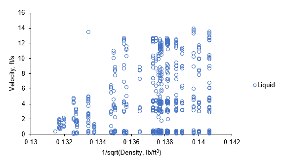
Figure 1 shows a scatter plot of the simulated results, the operating stable production rates in terms of the relationship between the liquid velocity and the reciprocal of the square root of the liquid density, for conditions where production was possible. For the various reservoir, fluid and pipe properties investigated, the velocities range from 0.0314 to 13.90 ft/s. Looking at the velocity distributions in Figure 1, there is no clear linear trend.
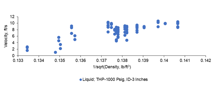
With further analyses of the simulation results, we observed a distinct linear trend between the velocities and the reciprocal of the square root of the density, when grouped into similar tubing head pressures and tubing sizes. Figure 2 represents a scenario for tubing head pressure of 1000 psig and tubing size of 3-in.
The empirical model, for erosion velocity calculation, was then created based on linear curve fitting using the least squares regression function in Microsoft EXCEL. Figures 3 and 4 are plots, for cases of tubing head pressure of 1000 psig and tubing size of 3 in., for liquid and gas, respectively.
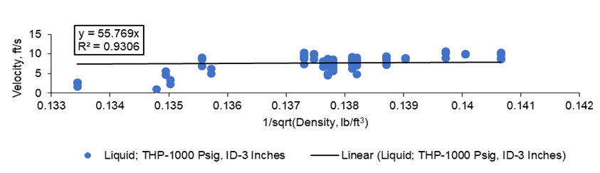
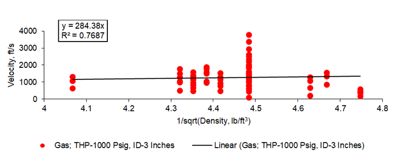
The results of the fitted data show that the R-squared value obtained is nearly close to unity for the liquid case and about 0.77 for the gas phase. The derived C-value is approximately 56 for the liquid phase and 284 for the gas phase, as can be seen in the equations in Figure 3 and 4, respectively. The C-value for the liquid phase is extremely low when compared to the empirical constant of 100 for clean services recommended by the America Petroleum Institute, the 14E (API RP 14E) equation. This could be as a result of the high gas-oil ratio of the fluids investigated, resulting in simulation results of high gas flow rates. The derived empirical constant, C-value, for the gas phase is however high, about 284.
Considering the tubing head pressures and the tubing sizes investigated, Table 1 shows the derived C-values for the ‘superficial’ liquid and gas cases, respectively. For both cases, the C-value increases as the tubing size and wellhead pressure increases.
| Tubing Head Pressures (THP), psig | Tubing Sizes (ID), ft | C-Values for Liquid Flow | C-Values for Gas Flow |
|---|---|---|---|
| 400 | 0.0833 | 2.67 | 11.963 |
| 400 | 0.1667 | 25.372 | 110.21 |
| 400 | 0.25 | 68.669 | 298.44 |
| 1000 | 0.0833 | 1.432 | 7.47 |
| 1000 | 0.1667 | 22.174 | 123.35 |
| 1000 | 0.25 | 55.769 | 284 |
| 1500 | 0.0833 | 0.7718 | 5.384 |
| 1500 | 0.01667 | 19.643 | 187.91 |
| 1500 | 0.25 | 38.141 | 256.47 |
Table 1: Derived _C_-values for liquid and gas cases.
Performing a multiple linear regression, with the constant set to zero, Equation 8 and 9 present the C-values (as a function of the tubing head pressure and the internal pipe diameter) for the ‘superficial’ liquid flow and gas flow, respectively.
$$ C _ {l} = - 0. 0 0 5 T H P + 2 0 9. 8 I D \tag {8} $$
$$ C _ {g} = 0. 0 1 7 7 T H P + 8 7 8. 8 6 I D \tag {9} $$
Considering two-phase multiphase flow scenario, the oil and gas flow rates after being converted into fluid flow velocities, Equation 10 was then used to obtain the mixture velocity, m U , for the multiphase flow.
$$ U _ {m} = U _ {s l} + U _ {s g} (1 0) $$
The mixture density was roughly estimated using Equation 11.
$$ \rho_ {m} = \lambda_ {l} \rho_ {l} + \lambda_ {g} \rho_ {g} (1 1) $$
where m ρ is the mixture density. lλ , g λ are fractions of the liquid and gas, respectively, as described in Equation 12 and 13.
$$ \lambda_ {l} = \frac {U _ {s l}}{U _ {m}} \tag {12} $$
sl l m U sg g m
$$ \left| \lambda_ {g} = \frac {U _ {s g}}{U _ {m}} \right| (1 3) $$
Figure 5 shows the fitted plot of the mixture velocity against the reciprocal of the square root of the mixture density. The derived C-value for the multiphase flow is approximately 846. This value is greatly higher than both the derived C-values for the ‘superficial’ liquid and gas flows. This is due to the increased flow rate, and the estimated mixture density may not be a true value for the multiphase flow. The derived C-value for the multiphase flow is also far greater than both the America Petroleum Institute, the 14E (API RP 14E), recommended value for clean service and the value of 183 developed by the Norwegian petroleum industry [14].
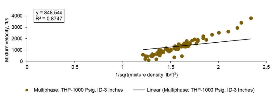
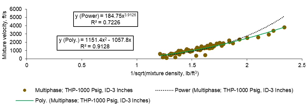
Looking at Figure 5, the best curve fitting might not be a linear relationship between the mixture velocity and the reciprocal of the square root of the mixture density. However, as the interest is to develop a generalized erosional velocity model, similar to the API 14E equation, the linear curve fitting relationship has been adopted. Other curve fitting models evaluated show that a second order polynomial equation best match the mixture velocity and the reciprocal of the square root of the mixture density (Figure 6).
| Tubing Head Pressures (THP), psig | Tubing Sizes (ID), ft | C-values for Multiphase Flow | |
|---|---|---|---|
| 400 | 0.0833 | 39.1 | |
| 400 | 0.1667 | 380.41 | |
| 400 | 0.25 | 1049.7 | |
| 1000 | 0.0833 | 22.46 | |
| 1000 | 0.1667 | 343.47 | |
| 1000 | 0.25 | 848.54 | |
| 1500 | 0.0833 | 14.344 | |
| 1500 | 0.01667 | 419.55 | |
| 1500 | 0.25 | 671.62 |
Table 2: Derived -values for the multiphase flow.
Table 2 presents the derived C-values for the multiphase flow. The C-value increases as the tubing size and wellhead pressure increases. Performing a multiple linear regression, with the constant set to zero, Equation 14 presents the C-value (as a function of the tubing head pressure and the internal pipe diameter) for multiphase flow in vertically producing pipes.
$$ C _ {m} = - 0. 0 3 0 7 6 T H P + 3 0 8 1. 8 1 I D \tag {14} $$
Therefore, the generalized erosional velocity model formulated for vertically producing multiphase flow wells can be expressed as:
0.03076 3081.81 e
| ρ m |
|---|
For a horizontal pipeline, the tubing head pressure in Equation 8, 9, 14 and 15 can be replaced with the upstream pressure of the pipeline under consideration.
Comparison of Results with Published Data
Predicted results, especially the C-factors, obtained from the newly developed models (Equation 8, 9, and 14) were compared with published data available in open literature with sufficient relevant information on the fluid flow conditions. In 2017, Ariana, et al. [1] designed and constructed four unique side stream pilot test units with 2 in. internal diameter for erosion/corrosion study. They investigated several flow rates in four fields. The average production and fluid data of one of the studied fields, Kangan Gas Field, is given in Table 3. The developed models in this work, Equation 9 for C-factor for the ‘superficial’ gas phase flow and Equation 12 for C-factor for the multiphase flow, predict approximate C-factors of 147 and 394, respectively. It shows that flow rate (likewise; pressure, pipe internal diameter, and fluid density) is an important parameter in the estimation of C-factor. These values could therefore be used to set limits for erosional velocity, for this reviewed case dominated by gaseous phase. Where the dominant phase is liquid, Equation 8 is to be applied. The C-factor estimated by the ‘superficial’ dominated phase flow can be considered to be safer (and reasonably conservative) for erosional velocity calculations.
| Internal Diameter, ft | Gas density, kg/m3 | Liquid density, kg/m3 | Gas Viscosity, cP | Liquid Viscosity, cP | Pressure, psi | Temperature, oC | U , sl m/s | U , sg m/s |
|---|---|---|---|---|---|---|---|---|
| 0.141 | 76.266 | 700.847 | 0.015 | 0.29 | 1324.62 | 54.74 | 0.093 | 29.02 |
Table 4: Average production and fluid data for kangan Gas Field.
The reported equivalent C-factors, considering Equation 1 - API RP 14E, for the different fluid flow rates investigated by Ariana, et al. [1] showed that all values lie in the range of 147 and 394. Mansoori [9] presented a field trial on four wells, to determine higher values of C-factor for use in the API 14E equation, on a real gas condensate field. The majority of wells were completed with 0.389 ft internal diameter tubing of N-80 grade material. Average mixture density of the four wells was 7.27 lb/ft3, average production rate equaled 63.62 MMscf/day. Comparison of actual velocity and API erosion velocity, with other relevant information for the four selected wells, indicated that the re-calculated C-factors using the API 14E but with the actual velocities are between 149 and 195. However, applying the newly developed models (Equation 9 and 14) considering only the second terms on the right- hand side of the equations as there is no information of the wellhead pressure, the estimated C-factor for the ‘superficial’ gas phase flow is 341 and that of the multiphase phase flow equals 1199. This means that even the subjected average production rate of 63.62 MMscf/day is conservative. The wells can withstand higher rates, even twice the subjected average production rates.
Panic, et al. [25] reported a velocity, just below the wellhead, of 121 ft/s (corresponded to a C-factor of 400) in a 0.583 ft outer diameter (OD) tubing and a velocity of 59 ft/s (corresponded to a C-factor of 200) in a 0.802 ft OD tubing with no failure producing from a gas condensate reservoir with pressure of 4500 psi and temperature of 110oC. Assuming that the values of the outer diameters are considered to be the internal diameters and the pressure of 4500 psi represents the wellhead pressure, the predicted C-factors by applying the newly developed models (Equation 9 and 14) are therefore 592 and 1658, respectively, for the 0.583 ft internal diameter pipe. For the 0.802 ft internal diameter tubing, the calculated C-factors are 784 and 2333, respectively. These values are quite higher than the reported corresponding C-factors for the gas-condensate wells. This implies that the produced rates are quite conserved, for the tubing sizes. This deduction is supported by the report of Ericson [11] that, “operators in the North Sea have used a -value of 726 for gas condensate wells”.
The Cannonball field, as reported by Healy, et al. [26], was brought on production in 2006 at a sustained rate in excess of 800 MMcf/day. The three gas wells - CAN01, CAN02 and CAN03, with a production tubing size of 7.625 in., had gas rates of 320, 295 and 255 MMcf/day, respectively. The flowing tubing head pressures were 3143, 2995 and 3592 psig, respectively. Gas gravity of 0.6137 was reported. Instead of using API RP 14E, a detailed erosion study was carried out using multiphase erosion prediction model and computational fluid dynamic (CFD) modeling for the technical assurance of an ultra-high rate of 400 MMcf/ day gas well completion design. As of 2008, there were no equipment, reliability nor sand issues. Applying the newly developed models (Equation 9 and 14), the predicted -factors for the gas well - CAN01 will be 613 and 1859, respectively. The C-factor from the ‘superficial’ gas flow, if used in the API RP 14E Equation (1) and a gas density of 0.6137 considered, will give a velocity that is one-third the reported gas rate of 320 MMcf/day. The equivalent velocity using the C-factor (Equation 14) for the multiphase flow, and considering the gas gravity of 0.6137, is very close to the reported rate.
Conclusion
The most common oil industry practice for sizing process piping, flow lines, pipelines, and tubing, is to limit the flow velocity to the maximum erosional velocity given by the API RP 14E equation. However, published reports showed that the evidence behind the basis of its development is not concrete. In addition, various values of the C-factor in the API RP 14E equation have been adopted based on field and laboratory experiences. In this study, stable operating production rates generated from more than a thousand of well performance simulations, with data from vertical wells in oil rim reservoirs in the Niger Delta, has been used to develop approximate erosional velocity models using the least square regression method. For the various reservoir, fluid and pipe properties investigated, fluid velocities range from a low value of 0.0314 to as high as 13.90 ft/s. Therefore, varying C-factors were obtained under the several simulated conditions under study. Based on the data analysed, linear trends were found for the C-factors and the tubing head pressures and the tubing sizes.
The development of erosional velocity models that incorporate the approximate quantifiable effects of both tubing head pressure and tubing size resulting to a robust generalisable model for single-phase liquid and gas flows and liquid-gas multiphase flows in pipes were then made. Comparison of results with published data were carried out, and the outcome showed that some tubing sizes can withstand velocities far greater than the recommended velocity by the API 14E. It is worthy to state that detailed erosion study using multiphase erosion prediction model, and computational fluid dynamic (CFD) modeling, if necessary, needs to be performed for the technical assurance of any predicted flow rate as actual velocities are known to fluctuate in the pipeline.
References
-
Ariana MA, Esmaeilzadeh F, Mowla D (2018) Beyond the Limitations of API RP-14E Erosional Velocity -A Field Study for Gas Condensate Wells Phys. Chem Res 6(1): 193-207.
-
American Petroleum Institute (1991) Recommended Practice Design and Installation of Offshore Production Platform Piping Systems, 4th (Edn.) API Recommended Practice 14E (RP 14E).
-
Salama MM, Venkatesh ES (1983) Evaluation of API- RP-14E Erosional Velocity Limitations for Offshore Gas Wells. Presented at the 15th Annual OTC in Houston, Texas.
-
Gamal A, Mohammed AAN, Hesham AMA, Aida Abdel Hafiez (2021) Erosional Velocity Limit for Several Oil Field Materials Based on Liquid Droplet Impingement. Proceedings of ICFD14: Fourteenth International Conference of Fluid Dynamics, Cairo, Egypt.
-
Arabnejad H, Shirazi SA, McLaury BS, Shadley JR (2014) A Guideline to Calculate Erosional Velocity due to Liquid Droplets for Oil and Gas Industry. SPE Annual Technical Conference and Exhibition, Amsterdam, The Netherlands.
-
Madani SF, Huizingab S, Esaklul KA, Nesic S (2019) Review of the API RP 14 Erosional Velocity Equation: Origin, Applications, Misuses, Limitations and Alternatives. Wear 426-427(Part A): 620-636.
-
Russell R, Nguyen H, Sun K (2011) Choosing Better API RP 14E C-Factors for Practical Oilfield Implementation, NACE international Conference, CORROSION, pp: 11248.
-
Esmaeilzadeh F (2004) Future South Pars Development may include 9 5/8-in Tubing. Oil Gas J 102: 53-57.
-
Mansoori H, Esmaeilzadeh F, Mowla D (2013) Case study: production benefits from increasing C-values. Oil Gas J 111: 64- 73.
-
Castle MJ, Teng DT (1991) Extending Gas Well Velocity Limits: Problems and Solutions. SPE Asia-Pacific Conference, Perth, Australia.
-
Ericson H (1988) Nipple, Lock, and Flow Coupling Recommendations and Sub-Assembly Description for North Sea wells. Priv Commun Nor Conoco.
-
Salama M (2000) An alternative to API 14E Erosional Velocity Limits for Sand-laden Fluids. J Energy Resour Technol 122(2): 71-77.
-
Vandeginste V, Piessens K (2008) Pipeline design for a least-cost router application for CO2 transport in the CO2 sequestration cycle. Int J Greenh Gas Control 2: 571- 581.
-
NORSOK P-002 standard (2014) Process System Design (Revision 1). Standards Norway (SN).
-
Svedeman SJ, Anorld KE (1994) Criteria for Sizing Multiphase Flowlines for Erosive/ Corrosive Service. SPE Production & Facility, pp: 74-80.
-
Nokleberg L, Sontvedt T (1995) Erosion in choke valves- oil and gas industry applications. Wear 186-187(Part-2): 401-412.
-
Springer GS (1976) Erosion by liquid impact. Scripta Publishing Company, pp: 246.
-
Ukpong SE, Livinus A (2023) Application of a Simulation Approach to Develop Erosional Velocity Correlation for Wells in Oil Rim Reservoirs in the Niger Delta. NAICE, Lagos, Nigeria.
-
Whitson CH, Brule MR (2000) Phase Behavior. SPE Monograph Series 20. Richardson, TX.
-
Fetkovich MJ (1973) The Isochronal Testing of Oil Wells. SPE Annual Meeting, Las Vegas, Nevada.
-
Griffith P, Wallis GB (1961) Two-Phase Slug Flow. Journal of Heat Transfer 83: 307-320.
-
Hagedorn AR, Brown KE (1965) Experimental Study of Pressure Gradients occuring during Continuous Two- Phase Flow in Small Diameter Vertical Conduits. J Pet Technol: 475-484.
-
Duns H, Ros NCJ (1963) Vertical Flow of Gas and Liquid Mixtures in Wells. Proceeding of the Sixth World Petroleum Congress, Frankfurt, pp: 22-PD6.
-
Gould TL, Tek MR, Katz DK (1974) Two-Phase Flow Through Vertical, Inclined, or Curved Pipe. J Pet Technol 26(8): 915-926.
-
Panic D, Leggoe J, House A (2009) Challenging Conventional Erosional Velocity Limitations for High Rate Gas Wells. CEEDWA, The University of Western Australia, Australia.
-
Healy JC, Martin J, McLaury B, Raynald Jagroop (2008) Erosion study for a 400 MMcf/D completion: Cannonball field, offshore Trinidad. SPE ATCE, Denver, Colorado, USA.
- Nigeria’s Vulnerability in the Face of Global Energy Policy
- A Simulation Study of Investigation of Optimum Oil Production Performance by Applying Various Gas Injection Methods in Oil Reservoir
- Characterization of Permo-Triassic Reservoirs through Thermal Maturity Assessment of Westphalian Source Rocks in the Cheshire Basin
- Influence of Microwax on the Rheological and Thermal Behaviour of a Wax Crude Oil
- Real-Time Monitoring and Performance Optimization of Steam Injection in Heavy Oil Reservoirs Using Fiber Optic Sensing and Integrated Predictive Simulation Models
- Rapid On-Site Determination of the Total Petroleum Hydrocarbon Content of Soils by Handheld Fourier Transform Near-Infrared Spectroscopy: Development of a Global, Site- and Scanner- Independent Calibration Model