Advancing Reservoir Performance Optimization through User-Friendly Excel VBA Software Development
This study addresses the pressing demand for streamlined field performance analysis within oil and natural gas development, which currently necessitates substantial expertise and time investment. The principal aim involves developing a user-friendly software tool dedicated to optimizing reservoir rendition. Leveraging the Havlena and Odeh material balance straight line equation form, this tool integrates a zero-dimensional reservoir model with Decline Curve Analysis. The implementation of this user-friendly software enables achievable material balance optimization by aligning cumulative produced fluid with historical production data, akin to the widely acknowledged concept of history matching in material balance analysis. This accomplishment not only facilitates further endeavors like pressure simulation and forecasting but also augments the comprehension of reservoir dynamics. The analysis incorporated three datasets: one modeled from L.P. Dake's textbook and two drawn from real-life reservoirs in the Niger Delta. Assessment of estimated water influx and cumulative oil production indicated minimal discrepancies between Np Real and Np model for these reservoirs. Consequently, material balance history matching for these reservoirs seems feasible. Achieving reservoir rendition optimization involved a Microsoft Excel VBA code consisting of two hundred and thirty-five (235) lines, meticulously designed to replicate MBAL functionality. The software demonstrated congruent outcomes with MBAL, affirming its reliability for history matching and enhancing reservoir performance. We strongly advocate the utilization of this software for optimizing reservoir performance across diverse global regions. Its capacity to streamline field analysis could significantly benefit the oil and natural gas industry.
Introduction
Forecasting the rendition of reservoirs support engineers in reserve estimation and develop a plan which requires a comprehensive knowledge of the features of the reservoir and optimization of production, to also create a model that will show the physical processes taking place in reservoirs [1, 2, 3]. In oil and gas reservoir development, projected field performance is the information required by oilfield workers that are into the design, risk, and decision-making process. Field performance analysis can require a substantial number of skills. Implementing the appropriate modeling approach is therefore the key to analyzing a field’s performance efficiently [4, 5]. Sophisticated and detailed models rely on the set of fluid and reservoir data that are available. Prediction of a field’s performance has to do with calculations of pressures, flow rates, cumulative productions, and expected production times using the available reservoir, production network, and production constraint data [6, 7, 8]. Every reservoir is made up of a unique arrangement of geometric form, rock properties, fluid properties and primary drive mechanisms. Though no two reservoirs are similar, they are categorized according to the primary recovery mechanism which they produce with. The performance characteristics of every producing mechanism are studied based on Decline rate of Pressure, Gas-oil ratio, Water production and Ultimate recovery [9, 10, 11]. The physical process behind material balance was reviewed and validated first by Schilthuis [9]. Odeh, et al. [12] put the equation into linear form making it simpler to understand and use. Plots were created considering the drive mechanism supporting the reservoir. Once a horizontal straight line is obtained in the plots, it means a purely depletion drive influence. If it deviates, then it’s not performing as anticipated which automatically suggests that other drive mechanisms effects are present. Coats, et al. [13] worked on the prediction of gas well performance. They investigated the gas well performance by developing a numerical model. Three field applications were conducted considering the effects of various parameters. The gas well performance was forecasted [14, 15, 16]. Miranda, et al. [17] in their work used cumulative reservoir withdrawals in place of the original fluid in place. DeSorcy [18] estimated the accuracy of each of the parameters. Galas [19] investigated an automated history matching system for the method by evaluating non- linear regression function and established that the boundary of matching parameters should not be overlooked. Esor, et al. [5] and Amudo, et al. [15] considered the application and methodology of the MBAL tool in developing connected oil and gas volumes in place. Bui, et al. [4] carried out their work to investigate the mature Samarang field’s reservoir compartmentalization using material balance analysis. They investigated the relationship between relative permeability curves and their effectiveness on history matching using the workflow of material balance analysis. Baker, et al. [20] provided a workflow process in Eclipse simulator. Mazloom, et al. [21] assessed the MB prognosis results from the models of single- and multi-tank. They discovered that the multi-tank model results were better than that of the single-tank model. Garcia, et al. [22] evaluated a meaningful parameter that disturbs material balance computation. His work showed the reservoir pressure and PVT data affects the OOIP calculation. Tarek [23, 24] stated in his work that MBE is used by reservoir engineers for future rendition forecast by continuously showing ways to optimally produce hydrocarbons in situ. Adeboye, et al. [14] used an enhanced model to forecast reservoir rendition. They stated that the parameters that govern decline must be understood. Mike, et al. [25] studied how reservoir rendition of reservoir changed with time. They stated in their work that the MBE is a handy tool for quickly defining reservoir drives, possible fluid contact, fluid-in-place for reservoirs and prediction of reservoir performance with time. Okotie, et al. [10] developed software called REPAT forecast reservoir rendition. MBE, expansion of Tarners method were utilized to produce the software which put into consideration aquifer influx and time. They discovered that water drive and fluid expansion drive supported the reservoir’s performance. Yong [26] made a method that showed reservoir variety and field development method change on the rendition of a reservoir. The time consumed by the new method is shorter than that of the tine reservoir simulation. Written computer programs known as software, are employed in performing this analysis that involves complex mathematical models [10, 27, 28, 29]. Most of the commercial software is very expensive and as such extremely difficult for students and researchers to purchase. With sound understanding of the physics behind reservoir analysis coupled with good mathematical and programming skill, one can design a software that can perform like or even better than most commercial software, in agreement with this vision, I thought it wise to develop a software using Microsoft Excel VBA that can perform Material balance optimization analysis.
Predicting Reservoir Performance
Four methods are used in reservoir performance rendition. They include volumetric, Decline Curve Analysis, Reservoir simulation and Material balance methods [2, 3, 23, 24, 30, 31].
Volumetric
Volumetric technique deals with the calculation of reservoir rock volume, the hydrocarbon in place contained in that rock volume and that which can be recovered. Important considerations are Rock Volume, Elevation of fluid contacts, Petrophysical parameters such as porosity, permeability, and Recovery factor [32, 33].
Decline Curve Analysis
Historically, Arps’ observed that fluid production rate declines exponentially with time stimulated emergence and further development of decline curve analysis [34]. Many researchers Agarwal, et al. [35] and Fetkovich’s, et al. [36] contributed to the improvement and extension of this method applicability.
Reservoir Simulation
Reservoir simulation is based on the methodology put into a certain approach, where specific mathematical relationships describe ongoing physical processes in the reservoir Odeh [12]. These descriptions, i.e., models, define the engineering tasks that will be solved, and parameters used. By its nature, any methodology is developed considering specific assumptions, stipulations, simplifications, and solving methods, which further establishes opportunities, requirements, and constraints for the implementation of the specific method [37].
Material Balance
The Material Balance equation is the relationship that exists between the average reservoir pressure and reservoir performance [30, 38, 39] (Figure 1).
![Figure 1: Material balance tank model assumption [2].](/fulltextimages/11761/fig_1.png)
Generalized Material Balance Equation
Generalized material balance equation is:
$$ \text{Total underground withdrawal} = \text{oil produced} + \text{gas} $$
produced+ water produced.
$$ G a s p r o d u c e d, G _ {p} = \left(N _ {p} R _ {p} - N _ {p} R _ {s}\right) B _ {g} $$ $$ = N _ {p} \left(R _ {p} - R _ {s}\right) B _ {g} $$ Withdrawal = ( ) 0 p p p s g p w N B N R R B W B + − + The generalized material balance equation becomes:
+ − = − + − + − + + + + − −
B N B R R B N B B R R B mNB B
( ) ( )( ) g p p s g o oi si s g oi gi
0 1 (1) c s c NB m P W W B s Ä
( ) ( ) w wi f oi e p w wi
1 1
Predicting Reservoir Future Performance as a Function of Time
Prediction of future performance as a function of time is achieved by combining MBE with a fluid-flow equation and Darcy’s equation. Predicting the reservoir’s future performance is conducted in two phases [25]. Phase one predicts production of hydrocarbon cumulative as it links to the decline in reservoir performance. Phase two is relating reservoir performance with time.
Two kinds of reservoir with their prediction techniques considered are Under-saturated oil reservoir and Saturated oil reservoir.
Under-Saturated Oil Reservoir
Cumulative production prediction involves a straightforward determination. The MBE is:
$$ N = \frac {N _ {p} B _ {o}}{B _ {o i} C _ {e} \ddot {A} P} (2) $$
p o oi e Where; 1
$$ C _ {e} = \frac {1}{S _ {o}} \left[ S _ {o i} C _ {o} + S _ {w i} C _ {w} + C _ {f} \right] $$ $$ C _ {e} = \frac {B _ {o} - B _ {o i}}{B _ {o i} \ddot {\mathrm {A}} P} $$ o oi e oi From Equation (2), cumulative production will be derived for any given pressure decline as:
$$ N _ {p} = \frac {N C _ {e} B _ {o}}{B _ {o i}} \ddot {A} P \tag {3} $$
e o p oi
Saturated Oil Reservoir
The three techniques for predicting primary recovery performance are The Tarner’s technique, The technique of Muskata and The Tracy’s technique [40, 41, 42]. Material Balance Equation as a Linear Equation [12] Equate:
( ) p o p s g p w F N B R R B W B = + − + Production $$ E _ {o} = \left(B _ {o} - B _ {o i}\right) + \left(R _ {s i} - R _ {s}\right) B _ {g} $$
Oil + originally dissolved gas $$ = \left(\frac {B _ {g}}{B _ {g i}} - 1\right) B _ {o i} \Rightarrow 1 $$ B E B B
1 g g oi gi Free gas expansion $$ E _ {f, w} = B _ {o i} \left(C _ {w} S _ {w i} + C _ {f}\right) \ddot {A} P / \left(1 - S _ {w i}\right) $$
Connate water + rock $$ \therefore F = N \left[ E _ {o} + m E _ {g} + (1 + m) E _ {f, w} \right] + W _ {e} B _ {w} \tag {4} $$ Depletion Drive: A reservoir having no initial gas cap where m=0 and negligible influx of water, rock compressibility and connate water (We=0, Ef,w=0), the equation degrades to:
o F NE = (Straight line) (5)
$$ F = N E _ {o} + W _ {e} \Rightarrow \frac {F}{E _ {o}} = N + \frac {W _ {e}}{E _ {o}} \tag {6} $$ e o e o o Water Drive: No initial gas-cap (m=0).
$$ F = N \left(E _ {o} + E _ {f, w}\right) + W _ {g} \tag {7} $$
But below bubble point, is negligible.
$$ \therefore F = N E _ {o} + W _ {e} \Rightarrow \frac {F}{E _ {0}} = N + \frac {w _ {e}}{E _ {o}} \tag {8} $$ e o e o
0 Gas-Cap Drive: No water drive, is negligible.
$$ \therefore F = N \left(E _ {o} + m E _ {g}\right) \Rightarrow \frac {F}{E _ {0}} = N + \frac {m N E _ {g}}{E _ {o}} \tag {9} $$ ( ) g o g o
0
Reservoir Drive Mechanisms
The drive mechanism is the energy responsible for transporting the hydrocarbon in the pore space of the reservoir to the wellbore. The common natural drive mechanism includes Depletion drive, Gas-cap drive, Water drive and Combination drive. Other drive mechanisms include Compaction drive, Imbibition and Gravity drainage drive [43, 44, 45] (Figure 2).
![Figure 2: Reservoir drive mechanisms [45].](/fulltextimages/11761/fig_2.png)
Reservoir Drive Indices
Each respective drive mechanism contributes to production. Therefore, reservoir Drive Index = individual production contribution total underground HC production [(B B ) (R R ) B ] s g oi si , [B (R R ) B ] o p s g N o Depletiondriven DDI N p − + − ∴ = + − (10) [(B B ) (R R ) B ] s g oi si , [B (R R ) B ] o p s g N o Depletiondriven DDI N p $$ \therefore D e p l e t i o n d r i v e n, D D I = \frac {N \left[ \left(\mathrm {B} _ {o} - \mathrm {B} _ {\mathrm {o i}}\right) + \left(\mathrm {R} _ {\mathrm {s i}} - 1\right) \right.}{N _ {p} \left[ \mathrm {B} _ {0} + \left(\mathrm {R} _ {\mathrm {p}} - \mathrm {R} _ {\mathrm {s}}\right) \right]} $$ (11) [(B B ) (R R ) B ] s g oi si , [B (R R ) B ] p s g o N o Depletiondriven DDI N p $$ \therefore D e p l e t i o n d r i v e n, D D I = \frac {N \left[ \left(\mathrm {B} _ {o} - \mathrm {B} _ {\mathrm {o i}}\right) + \left(\mathrm {R} _ {\mathrm {s i}} - \mathrm {R} _ {\mathrm {s}}\right) \mathrm {B} _ {\mathrm {g}} \right]}{N _ {p} \left[ \mathrm {B} _ {o} + \left(\mathrm {R} _ {\mathrm {p}} - \mathrm {R} _ {\mathrm {s}}\right) \mathrm {B} _ {\mathrm {g}} \right]} \tag {12} $$ [(B B ) (R R ) B ] s g oi si , [B (R R ) B ] o p s g N o Depletiondriven DDI N p $$ \therefore D e p l e t i o n d r i v e n, D D I = \frac {N \left[ \left(\mathrm {B} _ {o} - \mathrm {B} _ {\mathrm {o i}}\right) + \left(\mathrm {R} _ {\mathrm {s i}} - \mathrm {R} _ {\mathrm {s}}\right) \mathrm {B} _ {\mathrm {g}} \right]}{N _ {p} \left[ \mathrm {B} _ {\mathrm {o}} + \left(\mathrm {R} _ {\mathrm {p}} - \mathrm {R} _ {\mathrm {s}}\right) \mathrm {B} _ {\mathrm {g}} \right]} \tag {13} $$ DDI+SDI+EDI+WDI = 1.0 (14) The determination of each index shows the different contribution of each drive mechanism towards production and hence, shows the dominant drive mechanism.
Methodology
In this study, Microsoft Excel Visual Basic for Application combined with a tank model of zero dimensions was developed to predict reservoir performance. It is a powerful programming language embedded by Microsoft. The program is fixed in MS-Office applications i.e., MS-Word, MS-Excel, MS-Access. Many engineers use VBA to establish calculation subroutine suchlike menus, toolbars, worksheets, charts, etc Walkenbach [46]. This makes MS-Excel, which has VBA, a very advantageous platform for developing models and simulations. The main reason is that most engineers are acquainted with MS-Excel applications. Microsoft Excel is a user-friendly workbook that contains several worksheets. It is easily used for data analysis. It also provides some ability for engineering calculations and analysis [47]. Microsoft Excel is easily available to every Microsoft user and ridiculously cheap when compared to other domain based commercial software. Behind Excel spreadsheet is another environment used by its users to execute complex calculations on the worksheet. This environment is called Visual Basic Application, thus the name Excel VBA. Excel has inbuilt functions that users can leverage on while manipulating through their data but in a circumstance where the user wants a new functionality that did not come with Excel as inbuilt function, the user can navigate to the VBA environment and write some lines of code as shown in figure 3, that works as functions in Excel. Figure 3 shows the coding page of the software. Reservoir analysis is a key task in oil and gas exploration. During such analysis, hydrocarbon reservoirs are studied using some mathematical models. These models have large runtime and require a computer to perform such tasks faster, and accurately. With this technology, Engineers can design Excel to execute the needed task.
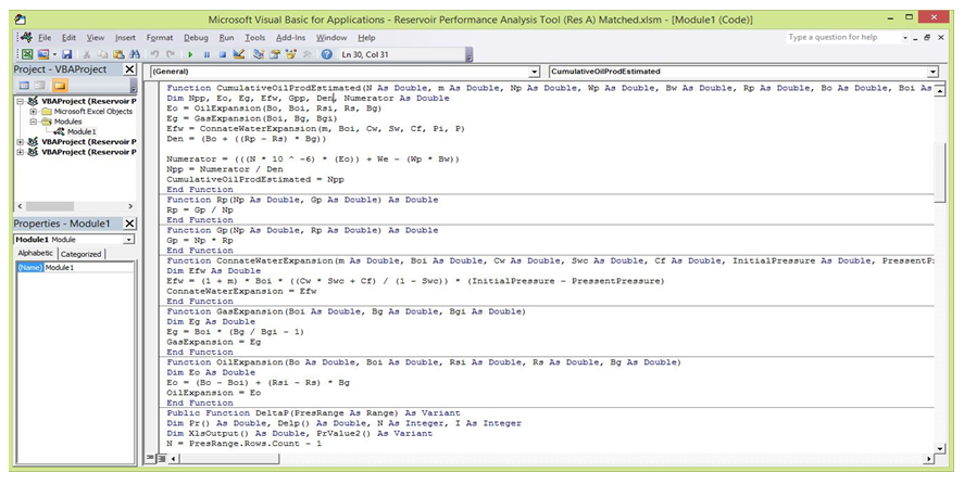
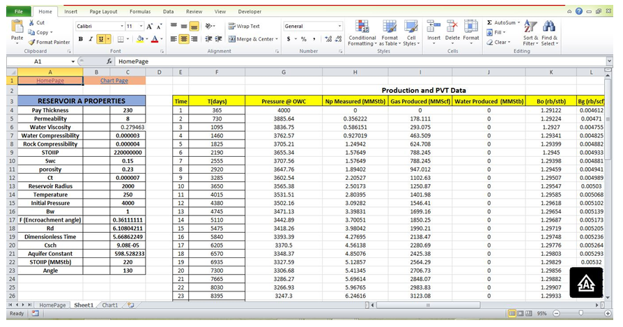
Figure 4 shows the interface of the Application. With this software, material balance optimization can be done on the cumulative produced fluid to obtain the history production data to match the model data. The common concept in material balance analysis is called history matching. When this is achieved, other activities like pressure simulation and forecasting can be executed to have more understanding and knowledge about the reservoir.

Functionality of the Excel Based Software
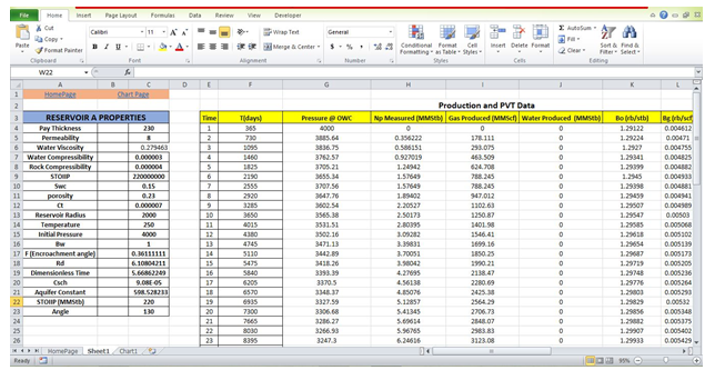
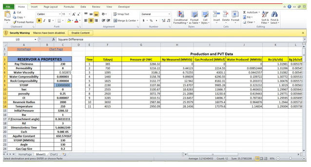
There are five major functions used during the setting up of the PVT and Production data used for the material balance optimization. DeltaP, TD, DimensionlessWaterInflux, WaterInfluxA and CumulativeOilProdEstimate. There are other functions in this Microsoft Excel software but these listed are the major ones. The appendix page has some of the functions. The reservoir, production and PVT data are displayed in the software as shown in Figure 5.
To perform the optimization after setting up the algorithm for sum of the square difference between Np Measured (oil reservoir) and Np Model; followed using the Microsoft Excel Solver to conduct the final optimization. This is what helps the software to history match these two parameters and try to get them match closely by changing some of the reservoir properties.
Reservoir engineering judgment comes in when selecting the right parameters to regress on. The reservoir engineer should be able to identify if the values he/she estimated is much or low that might not be the true value, but now that we have cumulative production from the reservoir, trying to align the models is like changing the parameters to suit what is observe from the reservoir.
Data Gathering and Acquisition
Three groups of data were used in carrying out this study; the first is a modeled data from the textbook by Dake [2] on water influx estimation while the second and third are real life data of reservoirs in Niger Delta. Reservoir A is a wedged shape reservoir. Initially the reservoir existed at Pb but no initial gas cap (m=0). Reservoir B is a linear- aquifer drive reservoir with strong water drive. It is still under depletion drive condition meaning it has no gas cap size (m=0). Reservoir Properties, Production, pressure and PVT data for reservoir A, B and C over a period are presented in Tables 1-9 respectively.
| Value | |
|---|---|
| Pay Thickness | 100 |
| Permeability | 200 |
| Water Viscosity | 0.55 |
| Water Compressibility | 0.000003 |
| Rock Compressibility | 0.000004 |
| STOIIIP | 312000000 |
| Swc | 0.05 |
| Porosity | 0.25 |
| Ct | 0.000007 |
| Reservoir Radius | 9200 |
| Temperature | 200 |
| Initial Pressure | 2740 |
| Bw | 1 |
| F (Encroachment angle) | 0.388888889 |
| Rd | 5.033837773 |
| Dimensionless Time | 5.668622493 |
| Csch | 9.08E-05 |
| Aquifer Constant | 6445.688667 |
| STOIIIP (MMStb) | 312 |
| Angle | 140 |
Table 1: Reservoir A Properties [2].
| T(days) | Pressure @ OWC | Plateau Pressure | Np_Measured (MMstb) | |
|---|---|---|---|---|
| 0 | 0 | 2740 | 2740 | 0 |
| 1 | 365 | 2500 | 2620 | 7.88 |
| 2 | 730 | 2290 | 2395 | 18.42 |
| 3 | 1095 | 2109 | 2199 | 29.15 |
| 4 | 1460 | 1949 | 2029 | 40.69 |
| 5 | 1825 | 1818 | 1883 | 50.14 |
| 6 | 2190 | 1702 | 1760 | 58.42 |
| 7 | 2555 | 1608 | 1655 | 65.39 |
| 8 | 2920 | 1535 | 1571 | 70.74 |
| 9 | 3285 | 1480 | 1507 | 74.54 |
| 10 | 3650 | 1440 | 1460 | 77.43 |
Table 2: Production and Pressure Data of Reservoir A.
| Time | T(days) | Pressure @ OWC | Plateau Pressure | Np_ Measured (MMstb) |
|---|---|---|---|---|
| 0 | 0 | 2740 | 2740 | 0 |
| 1 | 365 | 2500 | 2620 | 7.88 |
| 2 | 730 | 2290 | 2395 | 18.42 |
| 3 | 1095 | 2109 | 2199 | 29.15 |
| 4 | 1460 | 1949 | 2029 | 40.69 |
| 5 | 1825 | 1818 | 1883 | 50.14 |
| 6 | 2190 | 1702 | 1760 | 58.42 |
| 7 | 2555 | 1608 | 1655 | 65.39 |
| 8 | 2920 | 1535 | 1571 | 70.74 |
| 9 | 3285 | 1480 | 1507 | 74.54 |
| 10 | 3650 | 1440 | 1460 | 77.43 |
Table 3: PVT Data of Reservoir A.
| Property | Value |
|---|---|
| Pay Thickness | 230 |
| Permeability | 8 |
| Water Viscosity | 0.279463 |
| Water Compressibility | 0.000003 |
| Rock Compressibility | 0.000004 |
| STOIIP | 220000000 |
| Swc | 0.15 |
| Porosity | 0.23 |
| Ct | 0.000007 |
| Reservoir Radius | 2000 |
| Temperature | 250 |
| Initial Pressure | 4000 |
| Bw | 1 |
| F (Encroachment angle) | 0.361111111 |
| Rd | 6.108042106 |
| Dimensionless Time | 5.668622493 |
| Csch | 9.08E-05 |
| Aquifer Constant | 598.5282333 |
| STOIIP (MMStb) | 220 |
| Angle | 130 |
Table 4: Reservoir B Properties.
| Time | T(days) | Pressure @ OWC | Np Measured (MMStb) | Gas Produced (MMScf) | Water Produced (MMStb) |
|---|---|---|---|---|---|
| 1 | 365 | 4000 | 0 | 0 | 0 |
| 2 | 730 | 3885.64 | 0.356222 | 178.111 | 0 |
| 3 | 1095 | 3836.75 | 0.586151 | 293.075 | 0 |
| 4 | 1460 | 3762.57 | 0.927019 | 463.509 | 0 |
| 5 | 1825 | 3705.21 | 1.24942 | 624.708 | 0 |
| 6 | 2190 | 3655.34 | 1.57649 | 788.245 | 0 |
| 7 | 2555 | 3707.56 | 1.57649 | 788.245 | 0 |
| 8 | 2920 | 3647.76 | 1.89402 | 947.012 | 0 |
| 9 | 3285 | 3602.54 | 2.20527 | 1102.63 | 0 |
| 10 | 3650 | 3565.38 | 2.50173 | 1250.87 | 0 |
| 11 | 4015 | 3531.51 | 2.80395 | 1401.98 | 0 |
| 12 | 4380 | 3502.16 | 3.09282 | 1546.41 | 0 |
| 13 | 4745 | 3471.13 | 3.39831 | 1699.16 | 0 |
| 14 | 5110 | 3442.89 | 3.70051 | 1850.25 | 0 |
| 15 | 5475 | 3418.26 | 3.98042 | 1990.21 | 0 |
| 16 | 5840 | 3393.39 | 4.27695 | 2138.47 | 0 |
| 17 | 6205 | 3370.5 | 4.56138 | 2280.69 | 0 |
| 18 | 6570 | 3348.37 | 4.85076 | 2425.38 | 0 |
| 19 | 6935 | 3327.59 | 5.12857 | 2564.29 | 0 |
| 20 | 7300 | 3306.68 | 5.41345 | 2706.73 | 0 |
| 21 | 7665 | 3286.27 | 5.69614 | 2848.07 | 0 |
| 22 | 8030 | 3266.93 | 5.96765 | 2983.83 | 0 |
| 23 | 8395 | 3247.3 | 6.24616 | 3123.08 | 0 |
| 24 | 8760 | 3228.61 | 6.51371 | 3256.86 | 0 |
| 25 | 9125 | 3212.06 | 6.77893 | 3389.46 | 0 |
| 26 | 9490 | 3195.21 | 7.0423 | 3521.15 | 0 |
| 27 | 9855 | 3179.94 | 7.27854 | 3639.27 | 0 |
| 28 | 10220 | 3163 | 7.53836 | 3769.18 | 0 |
| 29 | 10585 | 3146.66 | 7.788 | 3894 | 0 |
| 30 | 10950 | 3129.82 | 8.04415 | 4022.07 | 0 |
| 31 | 11315 | 3109.13 | 8.28415 | 4142.07 | 0.028936 |
| 32 | 11680 | 3088.14 | 8.53215 | 4266.07 | 0.059586 |
| 33 | 12045 | 3067.3 | 8.78015 | 4390.07 | 0.091 |
| 34 | 12410 | 3047.2 | 9.02015 | 4510.07 | 0.122132 |
| 35 | 12775 | 3026.48 | 9.26815 | 4634.07 | 0.15504 |
| 36 | 13140 | 3006.46 | 9.50815 | 4754.07 | 0.18761 |
| 37 | 13505 | 2985.81 | 9.75615 | 4878.07 | 0.221995 |
| 38 | 13870 | 2965.19 | 10.0041 | 5002.07 | 0.257123 |
| 39 | 14235 | 2946.59 | 10.2281 | 5114.07 | 0.289503 |
| 40 | 14600 | 2926.01 | 10.4761 | 5238.07 | 0.326034 |
| 41 | 14965 | 2906.12 | 10.7161 | 5358.07 | 0.362088 |
| 42 | 15330 | 2885.58 | 10.9642 | 5482.07 | 0.400052 |
| 43 | 15695 | 2865.73 | 11.2042 | 5602.07 | 0.437484 |
| 44 | 16060 | 2845.24 | 11.4521 | 5726.07 | 0.476864 |
| 45 | 16425 | 2824.77 | 11.7001 | 5850.07 | 0.516957 |
| 46 | 16790 | 2804.98 | 11.9401 | 5970.07 | 0.556438 |
| 47 | 17155 | 2784.55 | 12.1882 | 6094.07 | 0.597924 |
| 48 | 17520 | 2764.81 | 12.4281 | 6214.07 | 0.638744 |
| 49 | 17885 | 2744.42 | 12.6761 | 6338.07 | 0.681605 |
| 50 | 18250 | 2724.07 | 12.9241 | 6462.07 | 0.725159 |
| 51 | 18615 | 2705.7 | 13.1481 | 6574.07 | 0.765106 |
| 52 | 18980 | 2685.39 | 13.3961 | 6698.07 | 0.809969 |
| 53 | 19345 | 2665.76 | 13.6361 | 6818.07 | 0.854039 |
| 54 | 19710 | 2645.5 | 13.8841 | 6942.07 | 0.900239 |
| 55 | 20075 | 2625.93 | 14.1242 | 7062.07 | 0.945597 |
| 56 | 20440 | 2605.73 | 14.3721 | 7186.07 | 0.993121 |
| 57 | 20805 | 2585.56 | 14.6201 | 7310.07 | 1.04131 |
| 58 | 21170 | 2566.08 | 14.8601 | 7430.07 | 1.08858 |
| 59 | 21535 | 2545.98 | 15.1082 | 7554.07 | 1.13808 |
| 60 | 21900 | 2526.57 | 15.3481 | 7674.07 | 1.1866 |
| 61 | 22265 | 2506.54 | 15.5961 | 7798.07 | 1.23738 |
| 62 | 22630 | 2486.55 | 15.8441 | 7922.07 | 1.28881 |
| 63 | 22995 | 2467.89 | 16.0761 | 8038.07 | 1.33751 |
| 64 | 23360 | 2447.98 | 16.3241 | 8162.07 | 1.39019 |
| 65 | 23725 | 2428.75 | 16.5641 | 8282.07 | 1.44177 |
| 66 | 24090 | 2408.92 | 16.8121 | 8406.07 | 1.4957 |
Table 5: Production Data of Reservoir B.
| Bo (rb/stb) | Bg (rb/scf) | Rp (scf/stb) | Rs (scf/stb) |
|---|---|---|---|
| 1.29122 | 0.0046118 | 0 | 500 |
| 1.29224 | 0.0047099 | 500 | 500 |
| 1.2927 | 0.0047546 | 499.999147 | 500 |
| 1.29341 | 0.0048249 | 499.9994606 | 500 |
| 1.29399 | 0.0048818 | 499.9983993 | 500 |
| 1.2945 | 0.0049332 | 500 | 500 |
| 1.29398 | 0.0048805 | 500 | 500 |
| 1.29459 | 0.0049414 | 500.001056 | 500 |
| 1.29507 | 0.0049894 | 499.9977327 | 500 |
| 1.29547 | 0.0050302 | 500.0019986 | 500 |
| 1.29585 | 0.0050684 | 500.0017832 | 500 |
| 1.29618 | 0.0051024 | 500 | 500 |
| 1.29654 | 0.0051388 | 500.0014713 | 500 |
| 1.29687 | 0.0051727 | 499.9986488 | 500 |
| 1.29719 | 0.0052053 | 500 | 500 |
| 1.29748 | 0.0052357 | 499.9988309 | 500 |
| 1.29776 | 0.0052645 | 500 | 500 |
| 1.29803 | 0.0052928 | 500 | 500 |
| 1.29829 | 0.0053199 | 500.0009749 | 500 |
| 1.29856 | 0.0053476 | 500.0009236 | 500 |
| 1.29882 | 0.0053752 | 500 | 500 |
| 1.29907 | 0.0054017 | 500.0008379 | 500 |
| 1.29933 | 0.005429 | 500 | 500 |
| 1.29958 | 0.0054554 | 500.0007676 | 500 |
| 1.2998 | 0.0054792 | 499.9992624 | 500 |
| 1.30003 | 0.0055036 | 500 | 500 |
| 1.30025 | 0.0055261 | 500 | 500 |
| 1.30048 | 0.0055513 | 500 | 500 |
| 1.30071 | 0.005576 | 500 | 500 |
| 1.30095 | 0.0056017 | 499.9993784 | 500 |
| 1.30125 | 0.0056337 | 499.9993964 | 500 |
| 1.30156 | 0.0056668 | 499.999414 | 500 |
| 1.30187 | 0.0057002 | 499.9994305 | 500 |
| 1.30217 | 0.0057329 | 499.9994457 | 500 |
| 1.30248 | 0.0057672 | 499.9994605 | 500 |
| 1.30279 | 0.0058009 | 499.9994741 | 500 |
| 1.30312 | 0.0058363 | 499.9994875 | 500 |
| 1.30344 | 0.0058722 | 500.0019992 | 500 |
| 1.30372 | 0.0059024 | 500.0019554 | 500 |
| 1.30406 | 0.0059401 | 500.0019091 | 500 |
| 1.30439 | 0.0059768 | 500.0018664 | 500 |
| 1.30474 | 0.0060153 | 499.9972638 | 500 |
| 1.30508 | 0.0060531 | 499.9973224 | 500 |
| 1.30543 | 0.0060927 | 500.0017464 | 500 |
| 1.30579 | 0.0061329 | 500.0017094 | 500 |
| 1.30614 | 0.0061725 | 500.001675 | 500 |
| 1.30651 | 0.006214 | 499.9975386 | 500 |
| 1.30688 | 0.0062548 | 500.0016093 | 500 |
| 1.30725 | 0.0062977 | 500.0015778 | 500 |
| 1.30764 | 0.0063413 | 500.0015475 | 500 |
| 1.30799 | 0.0063812 | 500.0015211 | 500 |
| 1.30838 | 0.0064262 | 500.001493 | 500 |
| 1.30877 | 0.0064704 | 500.0014667 | 500 |
| 1.30917 | 0.0065169 | 500.0014405 | 500 |
| 1.30957 | 0.0065626 | 499.997876 | 500 |
| 1.30999 | 0.0066106 | 500.0013916 | 500 |
| 1.31041 | 0.0066594 | 500.001368 | 500 |
| 1.31082 | 0.0067074 | 500.0013459 | 500 |
| 1.31125 | 0.0067579 | 499.9980143 | 500 |
| 1.31168 | 0.0068075 | 500.0013031 | 500 |
| 1.31212 | 0.0068597 | 500.0012824 | 500 |
| 1.31258 | 0.0069127 | 500.0012623 | 500 |
| 1.31303 | 0.0069665 | 500.0012441 | 500 |
| 1.31349 | 0.0070206 | 500.0012252 | 500 |
| 1.31394 | 0.0070741 | 500.0012074 | 500 |
| 1.31442 | 0.0071304 | 500.0011896 | 500 |
Table 6: PVT Data of Reservoir B.
| Property | Value |
|---|---|
| Pay Thickness | 230 |
| Permeability | 8 |
| Water Viscosity | 0.302872 |
| Water Compressibility | 0.000003 |
| Rock Compressibility | 0.000004 |
| STOIIP | 130000000 |
| Swc | 0 |
| Porosity | 0.25 |
| Ct | 0.000007 |
| Reservoir Radius | 2000 |
| Temperature | 210 |
| Initial Pressure | 3266.32 |
| Bw | 1 |
| F (Encroachment angle) | 0.361111111 |
| Rd | 3 |
| Dimensionless Time | 5.668622493 |
| Csch | 9.08E-05 |
| Aquifer Constant | 650.5741667 |
| STOIIP (MMStb) | 130 |
| Angle | 130 |
| Gas Cap Size | 0.2 |
Table 7: Reservoir C Properties.
| Time | T(days) | Pressure @ OWC | Np Measured (MMStb) | Gas Produced (MMScf) | Water Produced (MMStb) |
|---|---|---|---|---|---|
| 1 | 365 | 3266.32 | 0 | 0 | 0 |
| 2 | 730 | 3216.22 | 3.44123 | 2214.55 | 0.00852448 |
| 3 | 1095 | 3186.2 | 6.73255 | 4303.1 | 0.0442557 |
| 4 | 1460 | 3158.78 | 9.89839 | 6290.55 | 0.109722 |
| 5 | 1825 | 3132.77 | 12.942 | 8182.31 | 0.203372 |
| 6 | 2190 | 3107.86 | 15.8707 | 9985.28 | 0.323232 |
| 7 | 2555 | 3100.67 | 18.6263 | 11666.7 | 0.463631 |
| 8 | 2920 | 3072.79 | 21.2086 | 13230.6 | 0.619443 |
| 9 | 3285 | 3010.51 | 23.6457 | 14696.7 | 0.787383 |
| 10 | 3650 | 2987.86 | 25.9579 | 16079.4 | 0.964876 |
| 11 | 4015 | 2950.09 | 28.1436 | 17379.6 | 1.14834 |
Table 8: Production Data of Reservoir C.
| Bo (rb/stb) | Bg (rb/scf) | Rp (scf/stb) | Rs (scf/stb) |
|---|---|---|---|
| 1.31981 | 0.0053781 | 0 | 650 |
| 1.31396 | 0.0054502 | 643.5344339 | 637.663 |
| 1.31082 | 0.0054904 | 639.1486138 | 631.027 |
| 1.30772 | 0.005531 | 635.5124419 | 624.47 |
| 1.30476 | 0.0055708 | 632.2291763 | 618.186 |
| 1.3019 | 0.0056101 | 629.1644351 | 612.129 |
| 1.29967 | 0.0056415 | 626.3562812 | 607.397 |
| 1.29771 | 0.0056694 | 623.8318418 | 603.238 |
| 1.29595 | 0.005695 | 621.537954 | 599.502 |
| 1.2944 | 0.0057179 | 619.4414802 | 596.191 |
| 1.29304 | 0.0057382 | 617.5329382 | 593.297 |
Table 9: PVT Data of Reservoir C.
Results and Conclusion
The Microsoft excel software was developed first for each of the three different reservoirs. For unmatched Reservoir A, when the Np measured is 7.88 MMstb, the Np model is 7.93 MMstb. After history matching, the Np model gives a value of 7.91 MMstb with a square difference of 0.000767118 as clearly shown in Table 10 and Table 11 respectively.
| Np Measured (MMstb) | Np Model |
|---|---|
| (MMstb) | |
| 0 | 0 |
| 7.88 | 7.92996777 |
| 18.42 | 18.7664914 |
| 29.15 | 30.4817589 |
| 40.69 | 43.8164223 |
| 50.14 | 55.7345093 |
| 58.42 | 67.0134398 |
| 65.39 | 77.4142619 |
| 70.74 | 86.4666023 |
| 74.54 | 92.763234 |
| 77.43 | 101.264173 |
Table 10: Np Model and Np Real (Unmatched Reservoir A).
| Np Measured (MMstb) | Np Model (MMstb) | Square Difference |
|---|---|---|
| 0 | 0 | 0 |
| 7.88 | 7.90769689 | 0.000767118 |
| 18.42 | 18.45123718 | 0.000975761 |
| 29.15 | 29.23059583 | 0.006495687 |
| 40.69 | 40.85721089 | 0.027959481 |
| 50.14 | 50.36716779 | 0.051605204 |
| 58.42 | 58.679471 | 0.0673252 |
| 65.39 | 65.6818746 | 0.08519078 |
| 70.74 | 71.07091353 | 0.109503766 |
| 74.54 | 73.30750672 | 1.519039686 |
| 77.43 | 77.81607688 | 0.149055356 |
Table 11: Np Model and Np Real of Matched Reservoir A with their Square Differences.
The analysis of Reservoir A was done using the developed software depicted in Figure 6 which gives the correct values of DeltaP, Np model and Np measured with the respective time.
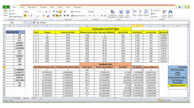
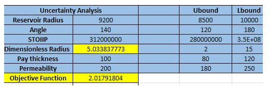
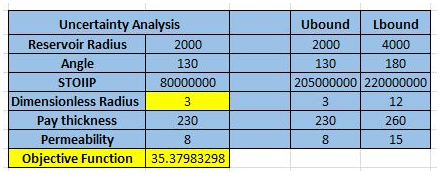
The uncertainty analysis of matched Reservoir A with STOIIP of 312MMstb gives a dimensionless radius of 5.03 alongside the objection function, pay thickness, permeability, angle, upper bound and lower bound values as shown in Figure 7.
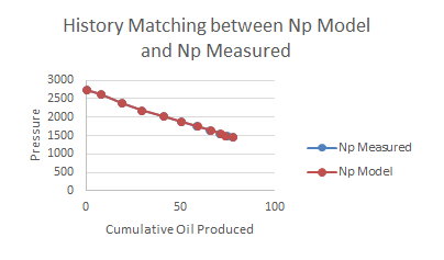
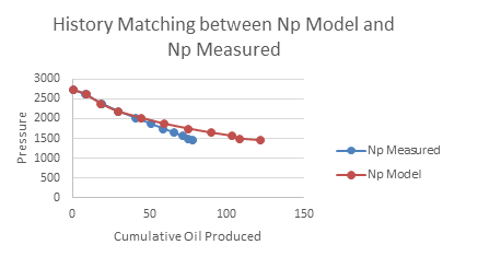
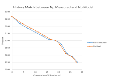
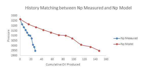
The history matching of the Np model and Np measured were carried out with their respective pressures. The plot of the matched reservoir A Np model value blended so perfectly with the Np measured as clearly depicted in Figure 8 and Figure 9.
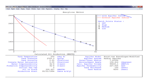
To test the accuracy of the developed software results, it was validated with MBAL. The blue in Figure 10 is with aquifer influx and the red line is without aquifer influx. It shows a high match points status.
Same process was repeated for reservoir B and C. The Np measured value of 9.78MMstb gives 10.04MMstb Np model with a square difference of 0.08 as shown in Table 12. Figure
11 shows the analysis page of Reservoir B indicating the reservoir properties, Production and PVT data.
| Np Measured (MMStb) | Np Model | Square Difference |
|---|---|---|
| 0 | 0 | 0 |
| 0.356222 | 0.4765031 | 0.014467535 |
| 0.586151 | 1.0530375 | 0.217982955 |
| 0.927019 | 1.6349144 | 0.501115831 |
| 1.24942 | 2.237253 | 0.97581412 |
| 1.57649 | 2.7808229 | 1.450417746 |
| 1.57649 | 2.8588125 | 1.644350891 |
| 1.89402 | 3.0873704 | 1.42408523 |
| 2.20527 | 3.5163371 | 1.718896884 |
| 2.50173 | 3.905998 | 1.971968721 |
| 2.80395 | 4.270592 | 2.151038763 |
| 3.09282 | 4.6047966 | 2.286073077 |
| 3.39831 | 4.9309404 | 2.348955917 |
| 3.70051 | 5.2441195 | 2.38273017 |
| 3.98042 | 5.534756 | 2.415960258 |
| 4.27695 | 5.8054107 | 2.336192163 |
| 4.56138 | 6.0639103 | 2.257597233 |
| 4.85076 | 6.3088486 | 2.126022497 |
| 5.12857 | 6.5419821 | 1.99773373 |
| 5.41345 | 6.7694534 | 1.838745229 |
| 5.69614 | 6.9910135 | 1.676697441 |
| 5.96765 | 7.2044221 | 1.529605184 |
| 6.24616 | 7.4150713 | 1.366353556 |
| 6.51371 | 7.6203424 | 1.224635173 |
| 6.77893 | 7.811036 | 1.065242869 |
| 7.0423 | 7.9956227 | 0.908824239 |
| 7.27854 | 8.1723812 | 0.798952042 |
| 7.53836 | 8.3484569 | 0.656256927 |
| 7.788 | 8.5257766 | 0.544314258 |
| 8.04415 | 8.7040871 | 0.435516994 |
| 8.28415 | 8.8809805 | 0.356206678 |
| 8.53215 | 9.0713449 | 0.290731161 |
| 8.78015 | 9.2652781 | 0.235349315 |
| 9.02015 | 9.4578839 | 0.191610943 |
| 9.26815 | 9.6513963 | 0.146877705 |
| 9.50815 | 9.8454615 | 0.113779074 |
| 9.75615 | 10.041408 | 0.081372128 |
| 10.0041 | 10.236701 | 0.054103401 |
| 10.2281 | 10.422759 | 0.037892257 |
| 10.4761 | 10.614188 | 0.019068193 |
| 10.7161 | 10.807077 | 0.008276873 |
| 10.9642 | 11.002109 | 0.001437091 |
| 11.2042 | 11.195719 | 7.19E-05 |
| 11.4521 | 11.389081 | 0.003971397 |
| 11.7001 | 11.585286 | 0.013182348 |
| 11.9401 | 11.778803 | 0.026016722 |
| 12.1882 | 11.973833 | 0.045953194 |
| 12.4281 | 12.168539 | 0.067371741 |
| 12.6761 | 12.361596 | 0.098912781 |
| 12.9241 | 12.558693 | 0.133522594 |
| 13.1481 | 12.747099 | 0.160801655 |
| 13.3961 | 12.936901 | 0.210863618 |
| 13.6361 | 13.129857 | 0.256281579 |
| 13.8841 | 13.322843 | 0.315009085 |
| 14.1242 | 13.516612 | 0.369163631 |
| 14.3721 | 13.711197 | 0.436793254 |
| 14.6201 | 13.906969 | 0.508556114 |
| 14.8601 | 14.100217 | 0.577422278 |
| 15.1082 | 14.294651 | 0.66186171 |
| 15.3481 | 14.488875 | 0.738267487 |
| 15.5961 | 14.682735 | 0.834235793 |
| 15.8441 | 14.880479 | 0.928564882 |
| 16.0761 | 15.075283 | 1.001633857 |
| 16.3241 | 15.26765 | 1.116085701 |
| 16.5641 | 15.460211 | 1.218571443 |
| 16.8121 | 15.655358 | 1.338052854 |
Table 12: Table of Np Model and Np Real of Matched Reservoir B with their Square Differences.
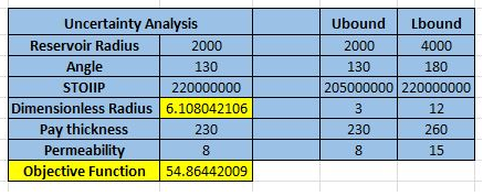
The uncertainty analysis yields a dimensionless radius of 6.10 with a STOIIP value of 220MMstb, reservoir radius of 2000 ft, pay thickness and the upper bound and lower bound values as shown in Figure 12.
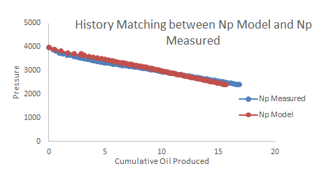
The history matching of the Np model and Np measured improved in the matched reservoir B plot compared to the unmatched reservoir B. The plots of pressure against the measured and model cumulative oil produced are shown in Figure 13 (Unmatched) and Figure 14 (Matched) respectively.
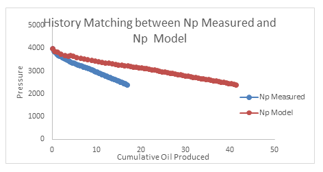
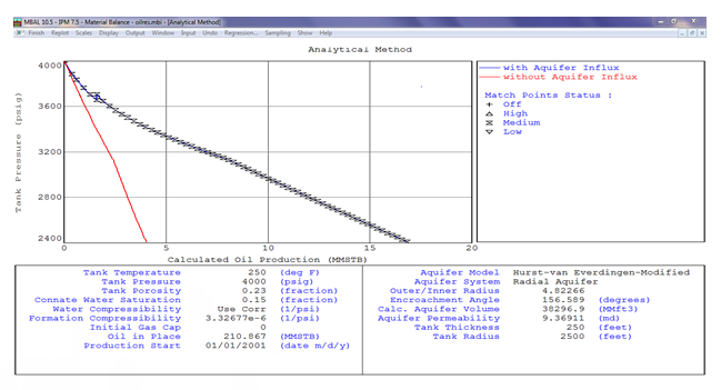
Figure 15 shows the software validation with MBAL. The Tank temperature is 250 deg F and tank pressure of 4000 psi. The calculated aquifer volume is 38296.9 MMft3 with aquifer permeability of 9.36911 md.
| Np Model | Np Measured (MMStb) | Square Difference |
|---|---|---|
| 0 | 0 | 0 |
| 5.971361026 | 3.44123 | 6.401563009 |
| 9.221039061 | 6.73255 | 6.192577805 |
| 12.36085017 | 9.89839 | 6.063710103 |
| 15.3245561 | 12.942 | 5.676573566 |
| 18.13870163 | 15.8707 | 5.143831381 |
| 20.32121837 | 18.6263 | 2.872748293 |
| 22.2272811 | 21.2086 | 1.037711176 |
| 23.97652918 | 23.6457 | 0.109447944 |
| 25.51907409 | 25.9579 | 0.192568183 |
| 26.84394561 | 28.1436 | 1.689101526 |
Table 13: Table of Np Model and Np Real of Matched Reservoir C with their Square Differences.
Reservoir A has no gas cap initially (m=0) and the compressibility term is negligible meaning that Eg and Efw term of the MBE will cancel out. Aquifer to reservoir radius value has a great impact in history matching for material balance. From LP Dake example, the first Np model estimation was done with aquifer to reservoir radius value of 10. The difference in the Np Model was extremely large but when we reduced it to 5, the two values matched each other. With the Excel VBA software, this was accomplished with ease. Reservoir B water-drive energy is strong like a typical Niger Delta reservoir, and still under depletion drive condition meaning no initial gas cap (m=0). Thus, material balance history matching of these two reservoirs will no longer be a difficult task as such. If the differences are too large, it will call for another water influx estimation or perhaps tedious iterative guessing on the aquifer parameters because uncertainties in the given data are as result of unknown aquifer parameters.
The optimization of reservoir performance by means of the 235 lines of code of the Microsoft Excel VBA mimics that of MBAL. The software gave results the same as MBAL, thus its usage for history matching is encouraged. For reservoir A, an example 9.2 in L.P. Dake, the difference in Np real and Np model were not significantly large. The Np model of the software follows the trend of the real when it was history matched. With little or no square differences. For reservoir B and C in this study, difference in Np real and Np model were not significantly large for real NIGER DELTA reservoirs. The Np model of the software follows the trend of the real when it was history matched. With little or no square differences. With the results obtained with this Excel VBA software, we can confidently say that the performance of any reservoir in any region can be enhanced using the obtained reservoir properties, production, and PVT data.
References
-
Old RE (1942) Analysis of Reservoir Performance. Am Inst Mining Eng 151(1): 86-98.
-
Dake LP (1978) Fundamentals of Reservoir Engineering. Elsevier Amsterdam, Netherlands, pp: 443.
-
Craft BC, Hawkins M (1991) Applied Petroleum Reservoir Engineering. 2nd(Edn), Prentice- Hall, New Jersey, pp: 448.
-
Bui T, Bandal M, Hutamin N, Gajraj A (2006) Material Balance analysis in Complex Mature reservoirs- Experience in Samarang Field, Malaysia. SPE Asia Pacific Oil & Gas Conference and Exhibition, pp: SPE 101138.
-
Esor E, Stefano D, Carlo M (2004) Use of Material Balance to Enhance 3D Reservoir Simulation: A Case Study. SPE Annual Technical Conference and Exhibition, Houston, Texas.
-
Lyon WC (1996) Standard Handbook of Petroleum and Natural Gas Engineering. Gulf publishing company 1: 1-1456.
-
Mea AC (2015) Predicting and Enhancing Reservoir Performance Using Material Balance Equation, case study of a multi tank model. Centre for Oil and Gas Technology.
-
Qiu K (2023) A practical analytical model for performance prediction in unconventional gas reservoir. Front Earth Sci 11: 1-9.
-
Schilthuis RJ (1936) Active Oil and Reservoir Energy. Trans 118(01): 33-52.
-
Okotie S, Onyekonwu MO (2015) Software for Reservoir Performance Prediction. Nigeria Annual International Conference and Exhibition, Lagos, Nigeria.
-
Ebere F, Minou R, Hui P, Vamegh R, Fadairo A, et al. (2022) The Bakken and Three Forks Formations Daily Crude Oil Production per Well Prediction Based on Support Vector Regression. Pet Petro Chem Eng J 6(4): 1-11.
-
Havlena D, Odeh AS (1963) The Material Balance as an Equation of a Straight Line. JPT 15(8): 896-900.
-
Coats KH, Dempsey JR, Henderson JH (1971) The use of vertical equilibrium in two-dimensional simulation of three-dimensional reservoir performance. SPEJ 11(1): 63-71.
-
Adeboye YE, Ubani CE, Oribayo O (2011) Prediction of reservoir performance in multi well systems using modified hyberbolic model. Journal of Petroleum Exploration and Production Technology 1: 81-87.
-
Amudo C, Walters MS, Reilly DI, Clough MD, Beinke JP, et al (2011) Best Practices and Lessons Learned in the Contraction and Maintenance of a Complex Gas Asset Integrated Production Model (IPM). Petroleum Experts, pp: 1.
-
Josephs RE, Porlles J, Tomomewo OS, Gyimah E, Ebere F (2023) Geo-Mechanical Characterization of a Well to Store Hydrogen. U.S Rock Mechanics/Geomechanics Symposium, Atlanta, Georgia, USA.
-
Miranda A, Raghavan R (1975) Optimization of The Material Balance Equations. J Can Pet Technol 14(04).
-
De Sorcy (1980) Proc of the 10th WPC 2: 269-277.
-
Galas CMF (1994) Confidence Limits of Reservoir Parameters by Material Balance. PETSOC Annual Technical Meeting, pp: SPE 94-035.
-
Baker RO, Chugh S, Mcburney C, Mckishnie (2006) History Matching Standards; Quality Control and Risk Analysis for Simulation. Petroleum Society’s 7th Canadian International Petroleum Conference, Canada.
-
Mazloom J, Tosdevin M, Frizzell D, Foley B, Sibley M (2007) Capturing Complex Dynamic Behavior in a Material Balance Model. International Petroleum Technology Conference, pp: IPTC 11489.
-
Garcia CA, Villa JR (2007) Pressure and PVT Uncertainty in Material balance Calculations. SPE Latin America and Caribbean Petroleum Engineering Conference, pp: SPE 107907.
-
Tarek A (2001) Reservoir Engineering Handbook. 2nd(Edn), Gulf Professional Publishing, pp: 484-780.
-
Tarek A, Paul DM (2005) Performance of oil reservoirs. Advanced reservoir engineering.
-
Mike PM, Beka FT, Kadana RI (2015) Predicting Reservoir Performance changes with Time. International journal for research in emerging science and technology 2(9).
-
Yong, Baozhu, Song B, Weimin Z, Qi Z (2016) Reservoir simulation history matching and waterflooding performance forecast for a large sandstone reservoir in Middle East (Russian). SPE annual Caspian Technical Conference and Exhibition.
-
Van Everdingen AF, Timmerman EH, McMahon JJ (1963) Application of Material Balance as an equation of Straight Line. Jou Pet Tech, pp: 896.
-
Smith CR, Tracy GW, Farrar RL (1992) Applied Reservoir Engineering. OGCI publication 2.
-
Falode OA, Udomboso C, Ebere f (2016) Prediction of Oilfield Scale formation Using Artificial Neural Network (ANN). Advances in Research 7(6): 1-13.
-
Dake LP (1994) The Practice of Reservoir Engineering. Revised Edition, Elsevier, pp: 78-79.
-
Dake LP (2001) The Practice of Reservoir Engineering. Developments in Petroleum Science 36.
-
(2006) Applied Reservoir Simulation-History Matching course material, Schlumberger, Denver and Houston.
-
Petrel 2010 Reservoir Engineering Course (2010) Schlumberger Publication.
-
Arps JJ (1945) Analysis of decline curves. Trans 160(01): 228-247.
-
Agarwal, Ram G, Al-Hussainy R, Ramey HJ (1965) The importance of Water influx in Gas Reservoirs. Journal of Petroleum Technology 17: 1336-1342.
-
Fetkovich MJ (1980) Decline curve analysis using type curves. J Pet Technol 32(06): 1065-1077.
-
Satter A, Iqbal GM, Buchwalter JL (2008) Practical Enhanced Reservoir Engineering. Pennwell Books, Tulsa.
-
Ogunyomi BA, Patzek TW, Lake LW, Kabir CS (2016) History matching and rate forecasting in unconventional oil reservoirs with an approximate analytical solution to the double-porosity model. SPE Res Eval Eng 19(01): 070-082.
-
Abed AA, Arslan CA, Sulaiman IN (2023) Study of the history matching and performance prediction Analysis Utilizing Integrated Material Balance Modeling in One Iraqi Oil Filed. Journal of Current Research on Engineering, Science and Technology 9(1): 47-62.
-
Tarner J (1944) How different size gas caps and pressure maintenance affect ultimate recovery. Oil Wkly, pp: 32- 36.
-
Muskat MM (1945) The production histories oil producing gas drive reservoirs. Jour Applied Physics 16: 147.
-
Tracy G (1955) Simplified form of the MBE. Trans 204: 243-246.
-
Ambastha AK, Aziz K (1987) Material Balance Calculations for Solution Gas Drive Reservoirs with Gravity Sagregation. 62nd Annual Technical Conference and Exhibition of the Society of Petroleum Engineers, Dallas, pp: 27-30.
-
Beggs D (2003) Production Optimization Using Nodal Analysis. 2nd(Edn), OGCI and Petroskills Publications, Tulsa, Oklahoma, pp: 150-153.
-
Lemonnier P, Bourbiaux B (2010) Simulation of Naturally Fractured Reservoirs. State of the Art: Part 2-Matrix- Fracture Transfers and Typical Features of Numerical Studies. Oil & Gas Science and Technology-Revue d’IFP Energies nouvelles 65(2): 263-286.
-
John Walkenbach (2007) Excel 2007 Bible.
-
Petroleum Expert IPM 7.5-MBAL 10.5 (2010).
- Nigeria’s Vulnerability in the Face of Global Energy Policy
- A Simulation Study of Investigation of Optimum Oil Production Performance by Applying Various Gas Injection Methods in Oil Reservoir
- Characterization of Permo-Triassic Reservoirs through Thermal Maturity Assessment of Westphalian Source Rocks in the Cheshire Basin
- Influence of Microwax on the Rheological and Thermal Behaviour of a Wax Crude Oil
- Real-Time Monitoring and Performance Optimization of Steam Injection in Heavy Oil Reservoirs Using Fiber Optic Sensing and Integrated Predictive Simulation Models
- Rapid On-Site Determination of the Total Petroleum Hydrocarbon Content of Soils by Handheld Fourier Transform Near-Infrared Spectroscopy: Development of a Global, Site- and Scanner- Independent Calibration Model