Data Analytics and Development of a Wellbore Cleaning Coefficient Model
In this study, wellbore cleaning coefficient (WCC) correlations were developed for three conventional coiled tubing sizes (2.375”, 2.625”, and 2.875”). These sizes correspond to roughness to internal (ε/D) ratios of 0.000460828, 0.000510637, and 0.000572517, respectively. Dimensional analysis, applying the Buckingham-π theorem and a database from 150 wells in the Spraberry formation in West Texas, was used. Key performance indicators (KPIs) that influence flow in a cased pipe around an object (coil tubing) were identified and employed in model development. These KPIs are (1) slick water density ( f ñ ), (2) slick water viscosity ( f μ ), (3) hydraulic diameter ( c t d - d ) between casing inner diameter (dc) and coil tubing outer diameter ( t d ), (4) average annular velocity ( v ) and (5) cleaning pressure gradient (ΔP) . The cleaning pressure gradient is the ratio of the circulating differential pressure (pu-pd) to measured depth (MD). A global model that relates WCC to the Euler number and the inverse of the Reynolds number was attempted at first. A low coefficient of multiple determination R2 of 0.626 was obtained. To better explain the physics of the cleaning process and improve the model fit, data segregation was performed by separating data into three data sets, a set for each ε/D ratio. R2 of 0.974, 0.945, and 0.877 were obtained. It was decided to separate the database further and create models that would be used to identify “clean” and “not clean” wellbores. These equations addressed operational conditions since in data partition threshold values of annular velocity, Euler and Reynolds numbers were applied to describe laminar and turbulent flow conditions. The predictive equations showed excellent degrees of fit with R2 of 0.979, 0.822, and 0.897, for clean wells for the three ε/D ratios, respectively. This study’s findings were also validated using cumulative debris versus elapsed time data from 12 Woodford wells.
Introduction
CT practices are becoming efficient in plug drillout operations in extended-reach laterals. These procedures have reduced operational costs, environmental exposure, and time to production. Service companies that did not use wipers, evaded short trips, optimized plug milling added benefits from bottomhole assemblies (BHAs), enhanced fluid monitoring techniques, and improved the overall system’s performance. However, despite these improvements more needs to be done to better optimize wellbore cleaning performance. The following literature review outlines efforts made to better understand the physics of cuttings transport problems. Authors developed different models, using computational fluid dynamics (CFD) and statistical analysis, but no attempts have been made to develop a wellbore cleaning coefficient model for drillouts in fractured wellbores. Li and Walker [1] performed 600 tests to study the effects of various parameters on cuttings transport in coiled tubing (CT) drilling. Software to predict cuttings transport was developed using the experimental data. In 2000, Cho et al. developed a three-layer model to predict and understand cuttings transport in a horizontal wellbore during CT drilling. The parametric model used parameters like drilling-fluid rheology, cuttings size/sphericity/concentration, wellbore geometry, eccentricity, and flow rate. Leising and Walton [2] looked at three different methods to explain wellbore- cleaning problems. The authors indicated that the usage of muddy water and viscous sweeps to periodically clean the casing is recommended. Li, et al. [3] collected flow-loop-test results and developed a computer program that predicted the time history of solids in-situ concentrations along wellbores. The software also predicted wellbore-cleaning times.
Gunawan and Rubiandini [4] investigated cuttings transport in horizontal CT throughout underbalanced drilling. The authors predicted hydrodynamic pressure, CT size, wellbore size, drilling fluids, and influx fluids. Kelessidis and Bandelis [5] discussed the effects of various parameters on efficient cuttings transport in horizontal concentric and eccentric annuli. The authors noted that flow ought to be turbulent in the annulus and that eccentricity led to a drastic decrease in cuttings-transport efficiency. Ramadan, et al. [6] studied the minimum transport velocity in a 4-m-long, 0.08-m pipe at inclinations of 90○ (horizontal) and 78○. The authors developed a minimum-transport-velocity model for drag-reducing polymers. Predictions were in total agreement with the experimentally measured data. Rolovic, et al. came up with an upgraded integrated system for wellbore-fill removal with CT. They monitored solids returns in real time and confirmed that the cleaning process progressed as planned.
In addition, Li and Wilde [7] investigated the effect of particle density and size on solids transport and wellbore cleaning with CT. They stated that the medium-sized particles (20/40 Carbolite) had the lowest transport efficiency in horizontal wellbores. New empirical correlations were developed to predict solids in-situ concentration, solids- carrying capacity, and optimal wiper-trip speed. Li and Luft studied the maximum rate of penetration (ROP) for various sand types at different deviated angles and water-flow rates for reverse-circulation cleanouts in a full-scale flow-loop- test facility. The authors stated that reverse-circulation cleaning is more efficient than forward circulation. They added that reverse water circulation would achieve the same cleaning efficiency as circulating a biopolymer with a 1% gel concentration. Using CFD, Osgouei, et al. [8]
studied cuttings transport in a horizontal annulus between concentric diameters of 0.047 and 0.074 m, respectively. The authors investigated the effects of the annular-flow rate and rate of penetration (ROP) on cuttings transport. The flow patterns in horizontal wells were also identified by the CFD software. Li and Luft [9, 10] presented a review of previous approaches to the study of solids transport in both drilling and well interventions with an emphasis on theoretical and experimental studies.
Song, et al. [11] investigated the characteristics and sand-sweeping efficiency of horizontal-wellbore cleanout by annular helical flow using CT. The effects of flow rate, cleaning distance, sand size, and nozzle assembly were discussed. Bizhani, et al. [12] conducted experimental work in a flow loop composed of a horizontal concentric annulus with a nonrotating straight inner pipe. It was found that cuttings transport with plain water was performed with lower flow rates and lesser pressure losses. Cuttings transport with polymers, on the other hand, took longer times as polymers tended to thicken and viscofy. Kamyab and Rasouli [13] investigated cuttings transport in a flow loop with two different simulated wellbore geometries (OD of the inner pipe and ID of the outer pipe were 0.0508 and 0.08 m and 0.0381 and 0.07 m, respectively). Results of the experiments were used to determine the minimum transport velocity to effectively bring all cuttings to surface.
Heydari, et al. [14] proposed a Eulerian multiphase model for cuttings transport. Using CFD, the effects of drillpipe rotation and eccentricity on cuttings transport in various horizontal annuluses were investigated. Busch, et al. [15] noted that -spaces can be used for scaling of process parameters as well as for quantitative comparison of results of cuttings transport. The authors added that the developed relationships could be used to improve real-time models. Huque, et al. [16] indicated that fluid rheology has a considerable effect on the minimum transport velocity and that turbulent flow is needed to effectively clean wellbores from cuttings. Khaled, et al. [17] presented a statistical model to predict hole-cleaning efficiency under different drilling conditions in deviated wells. Model findings indicated that the utilized model provided promising results in assessing cuttings buildup in deviated wells (20–90° from vertical). Yeo, et al. [18] studied hole cleaning in inclined wellbores. The CFD simulations looked at the variation of Reynolds number to critical velocity and critical pressure gradient.
The authors noted that developed correlations should use field data for validation. Wang, et al. [19] demonstrated that hole cleaning efficiency increases significantly with the drill pipe rotational rate, flow rate, and 6 RPM Fann dial reading. The authors used a combined CFD-discrete element technique simulation model to study the interaction between cuttings and drilling fluids. Chen, et al. [20] performed a simulation study on cuttings transport of wavy wellbore trajectories in extended-reach wellbores. To evaluate the effect of buildup rate on hole cleaning, a parametric analysis was performed. Results showed that wavy wellbores display greater risks of drilling complications as compared to conventional wellbores. A review of the existing literature on wellbore cleaning coefficient models, especially those applicable to fractured reservoirs, has been done. Gaps and limitations in the current knowledge as to the lack of a wellbore cleaning model for fractured reservoirs have been identified. Therefore, the objective of this study is to develop a wellbore cleaning coefficient model for fractured reservoirs, specifically focusing on the Spraberry Field in the Permian Basin of West Texas. Developing empirical cleaning coefficient equations can be crucial for optimizing drillouts cleaning procedures in such reservoirs. The next paragraph describes the geological and reservoir aspects of the Sperry Field.
Field Geology
The Spraberry Field is a large oil field. The Spraberry Trend is part of a greater oil-producing region known as the Spraberry-Dean Play located within the Midland Basin. Estimated reserves of the entire Spraberry-Dean unit surpass 10 billion barrels of oil. Horizontal wells are completed with several fractures to maximize the reservoir surface area to flow. In these wells, the plug n’ perf method is a conventional technique used for hydraulic fracturing. CT is used to mill out composite plugs to reestablish wellbore access and put wells into production, once fracturing is complete. To optimize the milling procedure, emphasis has been placed on designing better mill motors, bits, and plugs. As a result, mill motor life has increased, and bit design has substantially improved.
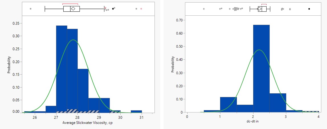
Figure 1a: Distribution plot of average slick water viscosity. Figure 1b: Distribution plot hydraulic diameter.
Nevertheless, no light has been shed on understanding solids transport in the wellbore during cleanout. Rules of thumb still overshadow the outcomes of pumping gels’ sweeps and decisions on the number of wiper trips needed to clean wellbores from milled composite plugs. These milling practices tend to leave behind variable amounts of debris in wellbores, causing stuck pipe incidents. These risks not only put at risk the safety of the operations but also add up to extra costs [21]. To perform data analysis and analytics, data of the identified KPIs have been extracted from many wells in the field. A complete data set comprising 150 wells would be used in the development of the empirical models.
Data Description of Model KPIs
A descriptive statistical summary or one-way analysis of the data for each KPI was generated. As shown in Table 1A in Appendix A, the summary includes the central tendency, dispersion, percentiles, and standard deviation of all available design parameters. When dealing with data, we must understand how the variables are distributed. As shown in Figures 1a, 1b, 2a, and 2b, the univariate distribution of each feature is plotted as a histogram. Most of the distributions are not normal, as some are skewed to the left and others are to the right. Statisticians investigate the possibility of data normalization. They use data transformation to delete outliers, reduce errors, and enable statistical models to perform better. Engineers, however, use three standard deviations around the mean, tend to keep most of the data and avoid deletion of outliers. These could have physical significance. Slick water density is 8.34 ppg. Figure 1a suggests that the average slick water viscosity data set is closely symmetrical. Figure 1b, however, indicates that the hydraulic diameter distribution is normal.
Figures 2a and 2b portray that average annular viscosity and pressure gradient data are normally distributed with no difference between means and medians.
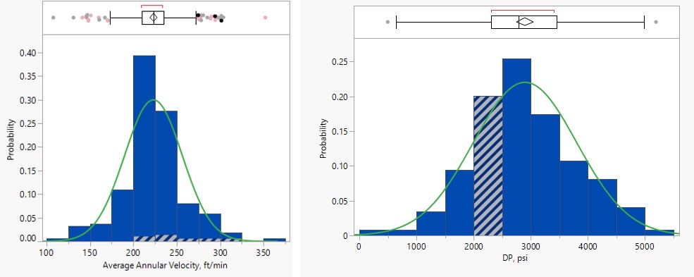
Figure 2a: Distribution plot of average annular velocity. Figure 2b: Distribution plot of pressure gradient.
No transformation would be done on either of the distributions since three standard deviations would be used to keep most of the data for model development. Eliminating outliers would force overfitting and would possibly discount data points that have physical significance.
Mathematical Model Development
Let ρ signify the density of the cleaning mixture stream (slickwater and cuttings) and let us assume that the geometry of the elemental volume (well) is approximated by a line of infinite length_l_ ; meaning that no boundary conditions are applied to the one-dimensional problem. Density at point and time is defined as ( ) ,t l ρ . Change of density over an arbitrary interval ( 1 2 , l l ) is:
l
2
1 l
2 ( ) $$ \int_ {l _ {1}} ^ {l _ {2}} \rho (t, l) d l \tag {1} $$
1 , It follows that the instantaneous density change at time is:
l l
2
2 ( ) $$ \int_ {l _ {1}} ^ {l _ {2}} \rho (t, l) d l = \int_ {l _ {1}} ^ {l _ {2}} \rho_ {t} (t, l) d $$ $$ \int_ {l _ {1}} ^ {l _ {2}} \rho_ {t} (t, l) d l \tag {2} $$
The cleaning liquid flux rate is also defined as:
1 ,
1 , ( ) ( ) ( ) ( )( ) 1 2 1 2 , , , , ct c ct q t l q t l t l A t l A A ν ν − = − − (3) where, ( ) 1 ,t l ρ , ( ) 1 , t l ν are flow rate and velocity of slick water entering interval( ) 1 2 , l l and ( ) 2 , q t l , ( ) 1 , t l ν are flow rate and velocity of slick water leaving the interval
( ) 1 2 , l l
, at time .t
ct
A is CT inner diameter cross-sectional
area and (
$$ \left(A _ {c} - A _ {c t}\right) \mathrm {t} \mathrm {t} \mathrm {t} t. A $$
is the hydraulic area between the casing
inner diameter and CT outer diameter.
where, $$ A _ {c t} = \pi d _ {c t} ^ {2} \mathrm {a n d} A _ {c} - A _ {c t} = \pi \left(d _ {c} ^ {2} - d _ {c t} ^ {2}\right) \tag {4} $$
with is the casing internal diameter and
c ct d d − is the hydraulic diameter.
Using mass conservation, the following formulation can be written:
l
2 ( ) ( ) ( )
$$ \int_ {l _ {1}} ^ {l _ {2}} \rho_ {t} (t, l) d l = q (t, l _ {1}) - q (t, l _ {2}) = - \int_ {l _ {1}} ^ {l _ {2}} q _ {l} (t, l) $$ $$ - \int_ {l _ {1}} ^ {l _ {2}} q _ {l} (t, l) d l \tag {5} $$
1 2 , , ,
1 , The change of sign implies that the liquid is loaded with more cuttings on the way out of the elemental volume. Finally, since the interval is arbitrary, density and flow rate must satisfy the following equation:
$$ q (t, l) = c \rho (t, l) \tag {6} $$
For some constant c, Equation 6 reduces to the following
linear one-dimensional transport equation:
t l c ρ ρ + = 0 (7)
where, ( ) ( ) 0 0, x x ρ ρ = with as initial density and length varies between the wellhead location (l=0) and MD (l = +∞), so no boundary conditions are needed. In the above cuttings transport model, terms that are accounted for include mixture (slick water + cuttings) flux densities and rates into the coiled tubing and out in the return line. These variables are not averages. They are time (in and out of the wellbore) and position (in and out of the wellbore) dependent.
In the developed mathematical model (Equation 7), KPIs that define (1) well geometry, (2) fluids properties, and (3) the dynamics of debris cleaning were utilized. These are:
- Measured Depth (MD) and hydraulic diameter (dc – dct) describing well geometry,
- Density ( f ρ ), defining slickwater properties, and
- Annular velocity (v ), explaining both the dynamics and the efficiency of the cleaning operation.
Slickwater viscosity ( f µ ), and cleaning pressure gradient ( P ∆ ) were added to better describe the slickwater properties, and cleaning efficiency, respectively. The mathematical relationship of the wellbore cleaning coefficient (WCC) as a function of these variables is therefore expressed as follows:
$$ \mathrm {W C C} = \mathrm {f i} \left(\rho_ {f}, \mu_ {f}, \mathrm {d} _ {\mathrm {c}} - \mathrm {d} _ {\mathrm {c t}}, v, \Delta \mathrm {P}\right) $$ (8) where fi signifies some unknown function.
Because of the complexity of finding a relationship between all parameters, it is believed that dimensional analysis could offer direct control in exploring relations among these variables. By applying the Buckingham-π theorem, the variables are combined into a set of dimensionless groups that reduce a complex problem to a study of relations among a smaller number of combined variables. As stated above, we considered 6 variables. Table 1 summarizes the symbols, units, and dimensions of the independent variables. Measured depth is imbedded in the cleaning pressure gradient, ∆P, term:
| Variable | Symbol | Units | Dimensions |
|---|---|---|---|
| Fluid density | ρf | lbm/ft³ | M/L³ |
| Fluid viscosity | μf | cp | M/LT |
| Hydraulic diameter | dc-dt | ft | L |
| Annular velocity | v | ft/s | L/T |
| Cleaning pressure gradient over the measured depth | ΔP | psia | M/TL³ |
Table 1: Buckingham- π model variables.
Using the Buckingham- π theory, we defined WCC as 1 π . 1 π is a slightly modified form of the Euler number (Eu). Euler is a dimensionless group that is used in the design of fluid flow. The number relates pressure to inertial forces; pressure forces seeking to push fluid through a restriction (casing/coiled tubing hydraulic diameter) and inertial forces depicting energy losses in the flow. A perfect frictionless flow corresponds to a Euler number of 0. The Euler number is defined as:
( )
2 p p d p p pressure forces E inertial forces u u d d ρ ρ $$ = \frac {p r e s s u r e f o r c e s}{i n e r t i a l f o r c e s} = \frac {\left(p _ {u} - p _ {d}\right) d _ {h} ^ {2}}{\left(\rho d _ {h} ^ {3}\right) \left(\frac {u ^ {2}}{d _ {h}}\right)} = \frac {p _ {u} - p}{\rho u ^ {2}} $$ u d h u d u (9)
2 2 3 ( ) h h
up : Average coiled tubing (upstream) pressure, N/m2,
dp Casing (downstream) pressure, N/m2,
h d : Hydraulic diameter of casing/coiled tubing, m, ρ : Fluid density, kg/m3, u : Fluid mean velocity, m/s,
2 π : Describes flow regimes. 2 π is defined as the inverse of the Reynolds number. The Reynolds number is a dimensionless number and is defined as the ratio of inertial to viscous forces. It is expressed as follows:
$$ R _ {e} = \frac {i n e r t i a l f o r c e s}{v i s c o u s f o r c e s} = \frac {u d _ {h}}{\nu} = \frac {\rho u d _ {h}}{\mu_ {f}} = \frac {\rho Q d _ {h}}{\mu_ {f} A} = \frac {W d _ {h}}{\mu_ {f} A} $$ (10) h h h h e f f f where: Q: Volumetric flow rate, m3/s, A: Casing/coiled tubing hydraulic cross-sectional area, m2, µ: Fluid dynamic viscosity, Pa·s = N·s/m2 = kg/(m·s), v: Kinematic viscosity (ν = /ρ), m2/s, W: Fluid mass flowrate, kg/s.
Reynolds number helps predict flow patterns for different fluid flow conditions. At low Reynolds numbers, fluid flow is likely to be laminar (sheet-like). At high Reynolds numbers, though, the fluid flow becomes turbulent. The used dimensionless groups and their definitions are summarized in Table 2.
| Group Name | Group Definition |
|---|---|
| π 1 | (d −d )×∆P c t ρ ×v2 f |
| π 2 | µ f (d −d )× v×ρ c t f |
Table 2: Models dimensionless groups.
No bivariate analysis would be done here since two dimensionless groups 1 π and 2 π have been identified.
Regression Analysis
A multi-regression analysis would be performed. All parameters impacting the wellbore cleaning coefficient would be utilized. The following form would be sought, where 2 π is an independent variable and 1 π is the dependent variable.
$$ \pi_ {1} = \beta_ {0} + \beta_ {1} ^ {*} \pi_ {2} (1 1) $$
In the multi-regression model, a relationship between the wellbore cleaning coefficient and all examined dimensionless parameters in the bivariate analysis would be sought. Only parameters that affect WCC would be considered in the parametric study. The goal here is to develop a unique empirical equation that can be used for operational purposes.
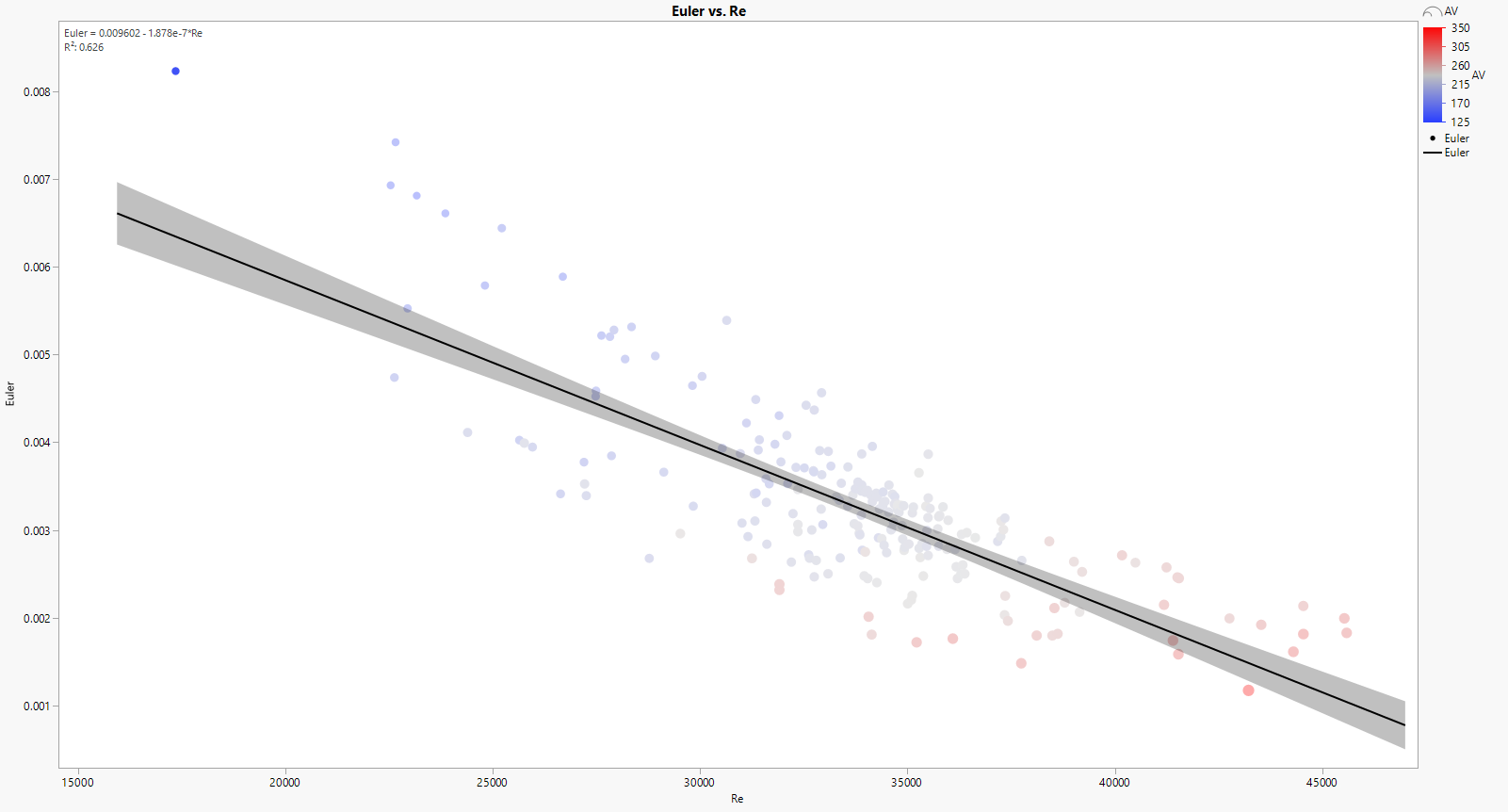
In Figure 3, Euler, 1 π was plotted as a function of the Reynolds number, 2 π , for all collected data (150 Spraberry wells), not clean and clean. The coefficient of multiple determination R2 was low at 0.626 for all roughness to internal (ε/D) ratios; ε/D = 0.000460828, ε/D = 0.000510637, and ε/D = 0.000572517.
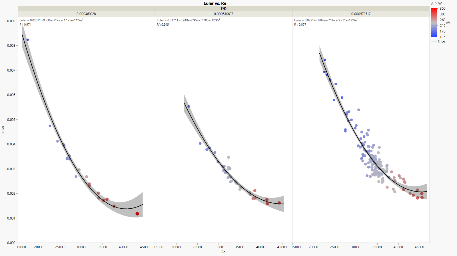
To better describe the dynamics of wellbore cleaning and hence improve the coefficient of multiple determination, it was decided to segregate the data. Three subgroups were created, considering each CT diameter (ε/D ratio). A descriptive statistical summary of collected data for coiled tubing sizes of 2.375”, 2.625”, and 2.875” is outlined in Tables 2A, 3A, and 4A in Appendix A. The summary includes minimums, maximums, medians, percentiles, and standard deviations of all design parameters that would be utilized in the development of cleaning models for the selected coiled tubing sizes.
Euler was plotted as a function of Reynolds number (Re) for each ε/D. Data segregation led to a better fit between the Euler and the Reynolds numbers (Figure 4). R2 of 0.974 and 0.945 were obtained for ε/Ds of 0.000460828 and 0.000510637, respectively. However, a lower R2 of 0.877 resulted for the ε/D ratio of 0.000572517.
Further data partitioning was done to come up with correlations that would be used for operational conditions. We identified operational conditions under which the well would be “clean” and others under which the well would not be clean; “not clean”. Data has therefore been separated into 2 subgroups: “not clean” and “clean”. “Not clean” is a term used for wells under laminar conditions that have not been cleaned properly. Laminar conditions pertain to an annular velocity lower than a threshold of 220 ft/s, a Euler greater than 0.003, and a Reynolds number lower than 29,000. “Clean”, on the other hand, applies to wells that are under turbulent conditions and have been suitably cleaned. Turbulent conditions affect wells cleaned with annular velocities of 240 ft/s and greater, a Euler of 0.003 and lower, and a Reynolds number of 29,000 and larger. Figure 5 depicts Euler as a function of Re for “not clean” and “clean” and an ε/D ratio of 0.000460828. The coefficient of determination showed an excellent fit with an R2 of 0.974. The obtained empirical equation is as follows:
$$ \mathrm {E u l e r} = 0. 0 2 0 7 1 - 9. 5 3 6 \mathrm {e} ^ {- 7} \times \mathrm {R e} + 1. 1 7 5 \mathrm {e} ^ {- 1 1} \times \mathrm {R e} ^ {2} \tag {12} $$
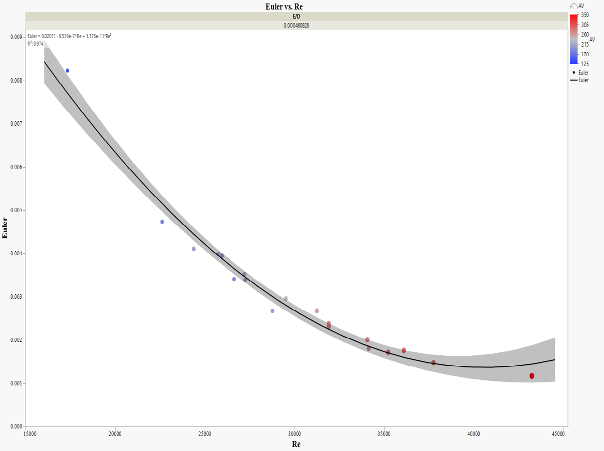
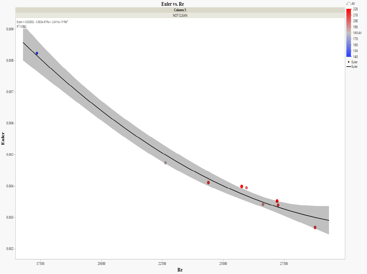
Figure 6 shows Euler as a function of Reynolds number for an ε/D ratio of 0.000460828 for “not clean” data only. The functional relationships yielded an R2 of 0.982. The resulting best-fit equation writes as:
$$ \mathrm {E u l e r} = 0. 0 2 8 0 2 - 1. 5 6 3 \mathrm {e} ^ {- 6} \times \mathrm {R e} + 2. 4 1 1 \mathrm {e} ^ {- 1 1} \times \mathrm {R e} ^ {2} \tag {13} $$
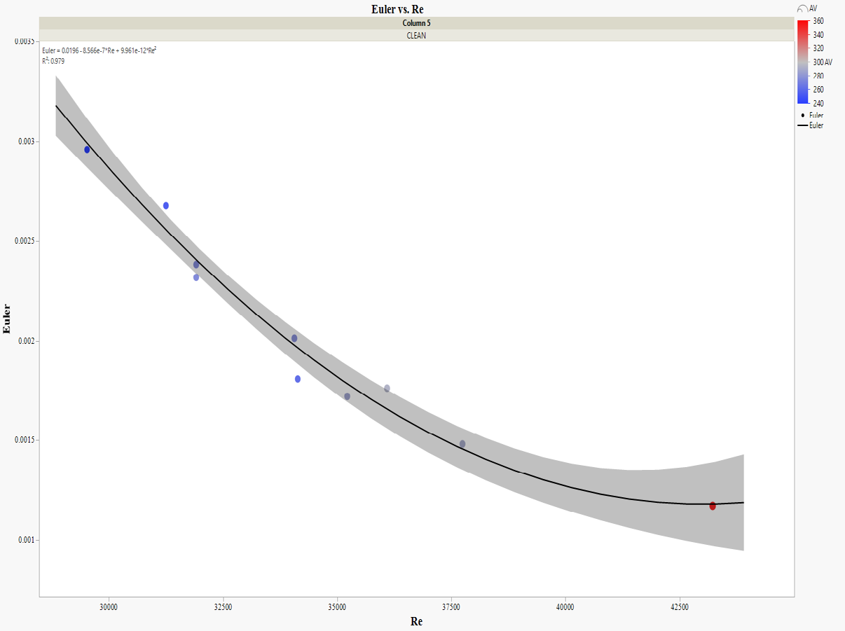
For “clean” data alone (Figure 7), the coefficient of multiple regression was found to be 0.979. The resulting empirical equation writes as:
$$ \mathrm {E u l e r} = 0. 0 1 9 6 - 8. 5 6 6 \mathrm {e} ^ {- 7} \times \mathrm {R e} + 9. 9 6 1 \mathrm {e} ^ {- 1 2} \times \mathrm {R e} ^ {2} \tag {14} $$
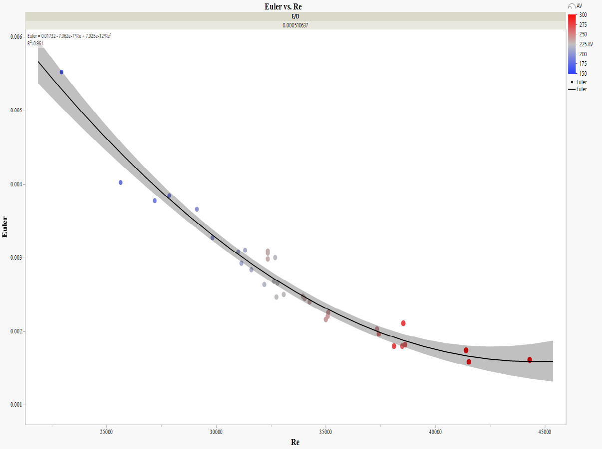
For ε/D = 0.000510637, “not clean” and “clean”, Figure 8 shows a coefficient of multiple regression of 0.961. The resulting empirical equation writes as:
7 12 2 Euler 0.01732 7.062e Re 7.925e Re − − = − × + × (15)
For “not clean” wells and for an ε/D ratio of 0.000510637, Figure 9 shows a better fit with an R2 value of 0.952. The derived observed equation is as follows:
$$ \mathrm {E u l e r} = 0. 0 2 4 9 6 - 1. 2 6 9 \mathrm {e} ^ {- 6} \times \mathrm {R e} + 1. 8 1 5 \mathrm {e} ^ {- 1 1} \times \mathrm {R e} ^ {2} \tag {16} $$
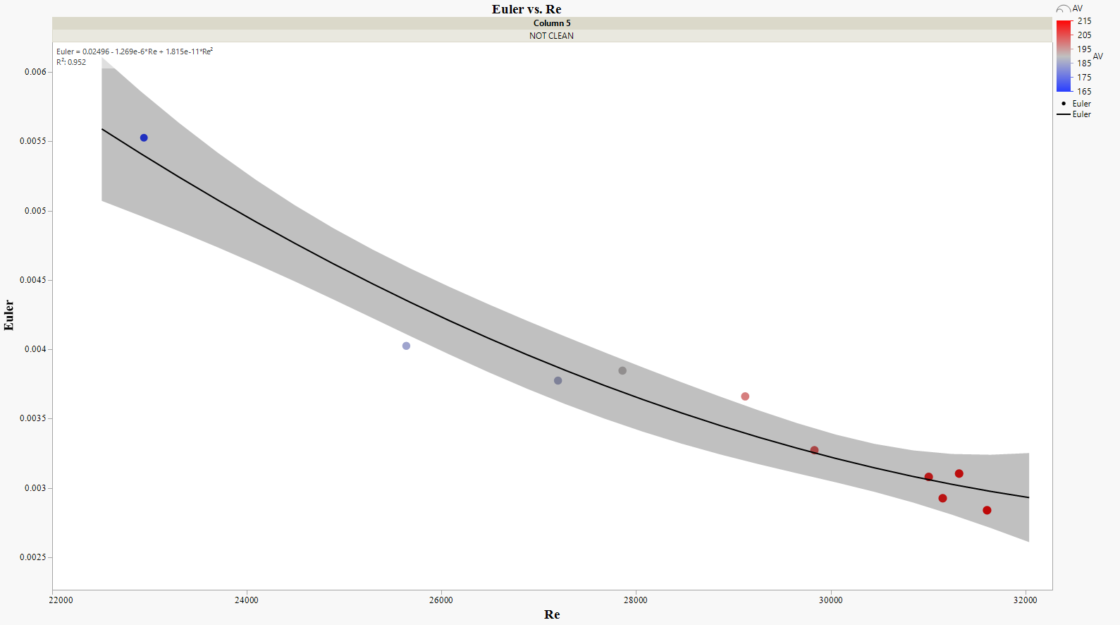
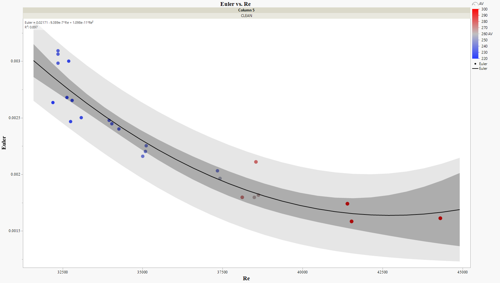
Figure 10 depicts Euler as a function Reynolds number for "clean" wells using an ε/D ratio of 0.000510637. The resulting coefficient of multiple determination R2 was found to be 0.897. The resulting empirical formulation is expressed as follows:
7 11 2 Euler 0.02171 9.389e Re 1.098e Re − − = − × + × (17)
In Figure 11, Euler was expressed as a function of Reynolds for “clean” and “not clean” using an ε/D ratio of 0.000572517. A coefficient of multiple determination R2 of 0.865 was estimated. The derived empirical equation writes as follows:
$$ \mathrm {E u} = 0. 0 1 9 0 3 - 7. 3 7 2 \mathrm {e} ^ {- 7} \times \mathrm {R e} + 7. 9 3 \mathrm {e} ^ {- 1 2} \times \mathrm {R e} ^ {2} \tag {18} $$

Figure 12 shows Euler as a function of Reynolds for “not clean” using an ε/D ratio of 0.000572517. An R2 value of 0.830 was found. The derived empirical model is expressed as follows:
7 12 2 Eu 0.01757 6.379e Re 6.602e Re − − = − × + × (19)

In Figure 13, Euler was plotted as a function of Reynolds for “clean” using an ε/D ratio of 0.000572517. The resulting R2 was found to be 0.848. The derived empirical equation writes as follows:
$$ \mathrm {E u} = 0. 0 1 3 4 6 - 4. 5 4 \mathrm {e} ^ {- 7} \times \mathrm {R e} + 4. 3 6 7 \mathrm {e} ^ {- 1 2} \times \mathrm {R e} ^ {2} \tag {20} $$

The following table summarizes derived empirical models for turbulent “clean” conditions for different roughness to coiled tubing diameter, ε/D, ratios. These equations would be benchmarked against data from other wells.
| ε/D | Derived Equations | R2 |
|---|---|---|
| 0.000460828 | Eu =0.0196−8.566e−7×Re+9.961e−12×Re2 | 0.979 |
| 0.000510637 | Eu =0.0217−9.389e−7×Re +1.098e−11×Re2 | 0.897 |
| 0.000572517 | Eu =0.01346−4.54e−7×Re+4.367e−12×Re2 | 0.848 |
Table 3: Derived models for “clean” wells.
Model Validation
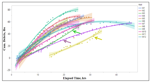
14 wells from the Woodford formation in the Permian Basin were used for model validation. Figure 14 depicts cumulative debris as a function of cleaning elapsed time, for the 14 wells. A steady increase (a nearly linear curve) in debris recovery indicates that these wells (9 out of 14) were cleaned effectively. Higher velocities with a Reynolds number larger than 29,000 contributed to continuous debris’ removal. The three curves (indicated by arrows) with a gentle slope and lower cumulative debris are for wells with lower annular velocities (less than 240 ft/s). These wells were not scrubbed successfully.
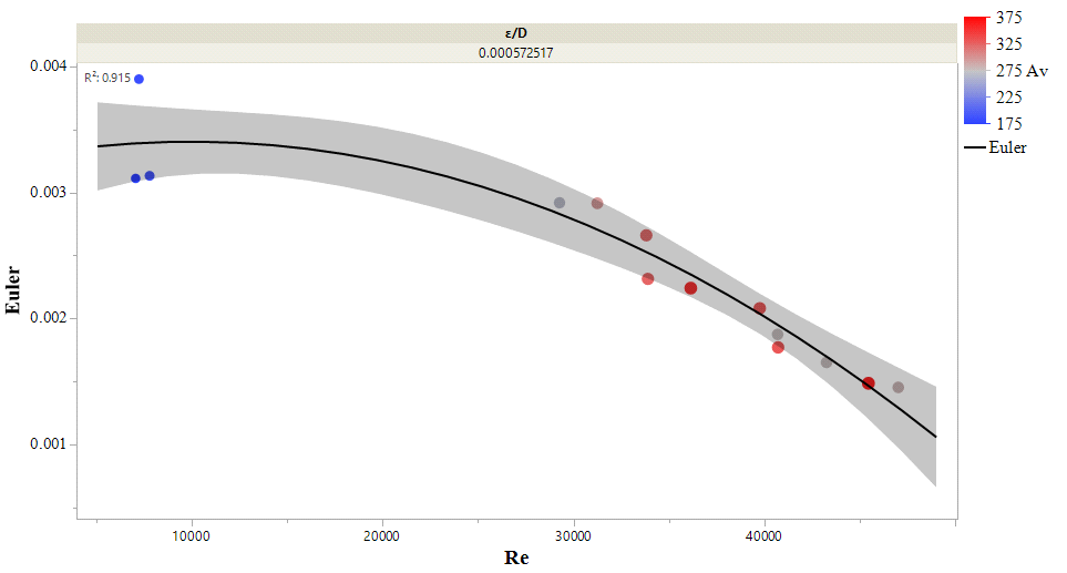
As depicted in Figure 15, Euler, and Reynolds numbers as well as annular velocity for the Woodford wells were all overlain on the same graph to identify “clean” and “not clean” wells and validate the study findings. The curve shows that only three wells (blue dots with lower Reynolds numbers) were not clean, the other 9 wells validated conclusions that wells with a Euler below 0.03 and a Reynolds number above 29,000 were cleaned efficiently.
Conclusions
Empirical equations that would be used to assess well cleaning in fractured wells have been developed. A global model using all data has been created to examine the relationship between Euler and Reynolds numbers at different annular velocities. The derived model showed a low coefficient of determination with an R2 of 0.626. Data segregation for three roughness to internal coiled tubing ratios (ε/D) of 0.000460828, 0.000510637, and 0.000572517 led to model improvement and better data fit. For an ε/D ratio of 0.000460828, the empirical equation gave an R2 of 0.979. As for the ratios ε/D of 0.000510637 and 0.000572517, the coefficient of multiple determination R2 was determined at 0.822 and 0.897, respectively.
It was concluded that collective metrics of annular velocity, Euler, and Reynolds numbers can be used to assess well-cleaning conditions. It was also established that for turbulent conditions; at annular velocities of 240 ft/s and greater, at a Euler of 0.003 and lower, and at Reynolds numbers of 29,000 and larger, cleaning becomes efficient, and the probability of stuck pipe and other operational inefficiencies are hindered. Collected debris from 12 Woodford wells has been used to validate the developed empirical equations and confirm the study findings.
Acknowledgements
The author and co-authors would like to thank the management of Emerald Surf Sciences – Corporate, Shreveport, Louisiana for providing the necessary data to perform this work.
Competing Interests
The authors declare that they have no competing interests.
Availability of Data and Materials
The data supporting the conclusions of this paper are included within the paper. Any queries regarding these data may be directed to the corresponding author.
Code Availability (Software Application or Custom Code Used)
N/A
Consent for Publication
Authors have agreed to submit it in its current form for publication in the journal.
Ethics Approval and Consent to Participate
Not applicable. No test, measurements or experiments on animals were performed as part of this work.
Funding
This research was not funded.
References
-
Li J, Walker S (1999) Sensitivity Analysis of Wellbore Cleaning Parameters in Directional Wells. SPE/ICoTA Coiled Tubing Roundtable, Houston, Texas, USA.
-
Leising LJ, Walton IC (2002) Cuttings-Transport Problems and Solutions in Coiled- Tubing Drilling. SPE Drill & Compl 17(1): 54-66.
-
Li J, Walker S, Aitken B (2002) How to Efficiently Remove Sand from Deviated Wellbores with a Solids Transport Simulator and a Coiled Tubing Cleanout Tool. SPE Annual Technical Conference and Exhibition, San Antonio, Texas, USA.
-
Gunawan I, Rubiandini R (2002) Determining Cutting Transport Parameter in a Horizontal Coiled Tubing Underbalanced Drilling Operation. SPE Asia Pacific Oil and Gas Conference and Exhibition, Melbourne, Australia.
-
Kelessidis VC, Bandelis GE (2004) Flow Patterns and Minimum Suspension Velocity for Efficient Cuttings Transport in Horizontal and Deviated Wells in Coiled- Tubing Drilling. SPE Drill & Compl 19 (4): 213-227.
-
Ramadan A, Saasen A, Skalle P (2004) Application of the Minimum Transport Velocity Model for Drag-Reducing Polymers. J Pet Sci Eng 44 (3-4): 303-316.
-
Li J, Wilde G (2005) Effect of Particle Density and Size on Solids Transport and Wellbore Cleaning with Coiled Tubing. SPE/ICoTA Coiled Tubing Conference and Exhibition, The Wood- lands, Texas, USA.
-
Osgouei RE, Ozbayoglu EM, Fu TK (2013) CFD Simulation of Solids Carrying Capacity of a Newtonian Fluid Through Horizontal Eccentric Annulus. Fluids Engineering Division Summer Meeting, Incline Village, Nevada, Vol 1C.
-
Li J, Luft B (2014a) Overview Solids Transport Study and Application in Oil-Gas Industry-Theoretical Work. International Petroleum Technology Conference, Kuala Lumpur, Malaysia IPTC-17832.
-
Li, J, Luft B (2014b) Overview of Solids Transport Studies and Applications in Oil and Gas Industry–Experimental Work. SPE Russian Oil and Gas Exploration & Production Technical Conference and Exhibition, Moscow.
-
Song XZ, Zhang L, Huang Z, Li G (2014) Mechanism and Characteristics of Horizontal-Wellbore Cleanout by Annular Helical Flow. SPE Journal 19(01): 45-54.
-
Bizhani M, Corredor FER, Kuru E (2016) Quantitative Evaluation of Critical Conditions Required for Effective Wellbore Cleaning in Coiled-Tubing Drilling of Horizontal Wells. SPE Drill & Compl 31(3): 188-199.
-
Kamyab M, Rasouli V (2016) Experimental and Numerical Simulation of Cuttings Transportation in Coiled Tubing Drilling. J Nat Gas Sci Eng (29): 284-302.
-
Heydari O, Sahraei E, Skalle P (2017) Investigating the Impact of Drillpipe’s Rotation and Eccentricity on Cuttings Transport Phenomenon in Various Horizontal Annuluses using Computational Fluid Dynamics (CFD). J Nat Gas Sci Eng 156: 801-813.
-
Busch, A, Werner, B, Johansen, ST (2019) Cuttings Transport Modeling – Part 2: Dimensional Analysis and Scaling. SPE Drilling & Completion 35(1): 69-87.
-
Huque MM, Rahman MA, Zendehboudi S, Butt S, Imtiaz S (2021) Investigation of Cuttings Transport in a Horizontal Well with High-speed Visualization and Electrical Resistance Tomography Technique. J Nat Gas Sci Eng 92: 103968.
-
Khaled MS, Khan MS, Ferroudji H, Barooah A, Rahman MA, et al. (2021) Dimensionless data-driven model for optimizing hole cleaning efficiency in daily drilling operations. J Nat Gas Sci Eng 96: 104315.
-
Yeo L, Feng Y, Seibi A, Temani A, Liu N (2021) Optimization of hole cleaning in horizontal and inclined wellbores: A study with computational fluid dynamics. J Nat Gas Sci Eng 205: 108993.
-
Wang, G, Dong, M, Wang, Z, Ren, T, Xu, S (2022) Removing Cuttings from Inclined and Horizontal Wells: Numerical Analysis of the Required Drilling Fluid Rheology and Flow Rate. J Nat Gas Sci Eng 102: 104544.
-
Chen Y, Zhang H, Li H, Zou Y, Lu Z, et al. (2022) Simulation study on cuttings transport of the wavy wellbore trajectory in the long horizontal wellbore. J Nat Gas Sci Eng 215(Part B): 110584.
-
Bureau of Economic Geology (2023) Wolfberry and Spraberry Play of the Midland Basin.
- Nigeria’s Vulnerability in the Face of Global Energy Policy
- A Simulation Study of Investigation of Optimum Oil Production Performance by Applying Various Gas Injection Methods in Oil Reservoir
- Characterization of Permo-Triassic Reservoirs through Thermal Maturity Assessment of Westphalian Source Rocks in the Cheshire Basin
- Influence of Microwax on the Rheological and Thermal Behaviour of a Wax Crude Oil
- Real-Time Monitoring and Performance Optimization of Steam Injection in Heavy Oil Reservoirs Using Fiber Optic Sensing and Integrated Predictive Simulation Models
- Rapid On-Site Determination of the Total Petroleum Hydrocarbon Content of Soils by Handheld Fourier Transform Near-Infrared Spectroscopy: Development of a Global, Site- and Scanner- Independent Calibration Model