Development of A Neural Boosted Model and JSL Code to Identify “Clean” or “Not Clean” Wells - A West Texas Sperry and Oklahoma Woodford Fractured Wells Coiled Tubing Cleaning Case Study
In a previous study, wellbore cleaning coefficient (WCC) correlations for cleaned wellbores out of debris and bridge plug remnants were developed for three conventional coiled tubing sizes (2.375”, 2.625”, and 2.875”). The following key performance indicators (KPIs): (1) slick water density ( ) f ρ , (2) slick water viscosity ( ) f μ , (3) hydraulic diameter c t (d - d ) between casing inner diameter (dc) and coil tubing outer diameter (dt), (4) average annular velocity (v) and (5) cleaning pressure gradient ΔP across a measured depth (MD) were employed in the empirical models. The models addressed operational conditions under which fractured wells will be identified as whether “clean” or “not clean”. In this study, the database from 150 wells, in the Spraberry formation in West Texas, was used to develop a predictive model to identify status of cleaned fractured wells: whether “clean” or “not clean”? About 70% of the data (99 wells) was used for training and about 30% (51 wells) for validation. 14 wells from the liquids-rich shale Woodford formation (Oklahoma) were utilized for testing. Six predictive modeling tools were designed to validate the derived empirical correlations. These tools are (1) Fit Stepwise, (2) Neural Boosted, (3) Boosted Tree, (4) Decision Tree (Partition), (5) Generalized Regression Lasso, and K-Nearest Neighbors. In the predictive models, independent variables are the annular velocity (AV), the Reynolds’ Number (Re), the Euler’s Number (Eu), and the coiled tubing roughness to internal radius ratio (ε/D). The dependent variable is well status; “clean” or “not clean”. Jump Scripting Language (JSL) code was used to develop user-friendly software. The software would be utilized to identify the fractured wellbore status, whether “clean” or “not clean”. Operators would be able to use the code to identify working conditions for which completed fractured wells are “clean” out of fracturing debris and remnants of bridge plugs or “not clean”. Input parameters to the code are AV, Re, Eu, and ε/D.
Literature Review
Artificial intelligence (AI) is a procedure that uses advanced algorithms, simulating the human brain, to train data and predict future systems operation [1]. AI has been used extensively in the fields of engineering, economics, medicine, the military, and certain marine sectors [2]. Artificial neural networks (ANNs), adaptive neuro-fuzzy inference systems (ANFIS), functional networks (FN), and support vector machine (SVM) are among the algorithms used in the oil and gas industry [3]. Three layers commonly characterize the architecture of an ANN model. These are an input layer, hidden layer(s), and an output layer [4]. Many algorithms were utilized for the learning procedure and control of the neurons’ processing capabilities [5]. To optimize the model network and enhance prediction accuracy, a set of weights and biases are utilized [6].
Ali [7] listed examples that included seismic pattern recognition, permeability predictions, identification of sandstone lithofacies, drill bit diagnosis, analysis, and improvement of gas well production. The author noted that neural network technology helped in the analysis, prediction, and optimization of well performance, integrated reservoir characterization, and portfolio management. Rispler, et al. [8] presented a case history in which ANN technology was used to successfully manage tubing strings during coiled tubing (CT) fracturing operations. The authors used the CT pressure ratings, tensile strength, and fatigue to determine CT life and identify a safe operating envelope. The ANN model they established could predict erosional wall loss and quantify critical performance parameters for specific applications. Ahmadi [9] utilized the least square support vector machine (LSSVM), adaptive network- based fuzzy inference systems (ANFISs), and enhanced particle swarm optimization PSO-ANFIS tools to assess the equivalent circulating density (ECD) using mud initial density, pressure, and temperature. Other studies applied learning techniques to solve operational challenges and enhance systems performance Rolon, et al. [10]; Tariq, et al. [11]; Elkatatny, et al. [12]; Mousa, et al. [13]; Alsabaa, et al. [14]. AI has also been used in the identification of reservoir lithology [15], prediction of the pore and fracture pressures [16], estimation of PVT properties [17], evaluation of the oil recovery factor [18, 19], projection of depths to the base of cap rocks in drilled formations [20], prediction of the rate of penetration (ROP) for various drilled formations [21, 22, 23] determination of total organic carbon (TOC) content [24, 25, 26], approximation of the rock static Young’s modulus [27, 28, 29, 30], determination of rock failure parameters [31, 32], detection of downhole anomalies during lateral drilling [33], determination of drill bit wear from drilling parameters [34, 35, 36, 37, 38], and prediction of the real-time drilling fluids rheological properties [14, 17, 35, 36, 37, 38] used extensive data to build an ANN model that predicts equivalent circulating density (ECD) from surface drilling measurements. Three thousand five hundred and seventy (3,570) data points were utilized to develop the model. Two thousand seven hundred and forty-three (2,743) data points were employed for training and eight hundred and twenty-seven (827) data points were used for testing. Only one hidden layer with 15 neurons was utilized for better prediction accuracy. Results indicated a correlation coefficient (R) of 0.99 and an average absolute percentage error (AAPE) of 0.24%. Model testing yielded an R of 0.98 and an AAPE of 0.3%.
In the cited literature, there was no mention of empirical equations or neural networks that have been developed to identify the status of clean fractured wellbores. The goal of this study is to use 6 neural predictive tools to validate bridge plugs cleaning coefficient correlations that have been derived in a previous study and develop a JSL code. The code is user-friendly software that can be employed to identify operational conditions for which fractured wellbores are “cleaned” off fractured formation debris and remnants of bridge plugs.
Data Description and Statistical Analysis
This study utilized real-time data (RTD) that was collected during cleaning operations in wellbores around the country. The original data deck contained statistics from 5000 wells, in Louisiana, Texas, Wyoming, Oklahoma, North and South Dakota, Colorado, and New Mexico. Most of the wells, 500, were drilled in Texas. The mined data were preprocessed using JMP and only 150 wells had complete datasets. The data included measured slick water density (ρf), slick water viscosity (µf), hydraulic diameter (dc-dt), average annular velocity (v), and cleaning pressure gradient (∆P).
Using the Buckingham-π theory, two dimensionless groups π1 and π2 were identified. π1, the well cleaning coefficient (WCC), is a slightly modified form of Eu. π2 is the inverse of _R_e.
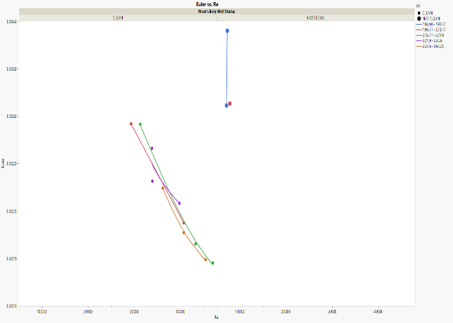
In the performed regression analysis, three models for “clean wells” for three roughness to coiled tubing diameter, ε/D ratios, have been developed. These empirical models that have been benchmarked against data from 14 wells from the Woodford formation are summarized below:
| ε/D | Derived Equations | R2 |
|---|---|---|
| 0.000460828 | −7 −12 2 Eu = 0.0196 - 8.566e ×Re+9.961e ×Re | 0.979 |
| 0.000510637 | −7 −11 2 Eu = 0.0217 - 9.389e ×Re+1.098e ×Re | 0.897 |
| 0.000572517 | −7 −12 2 Eu = 0.01346 - 4.54e ×Re+ 4.367e ×Re | 0.848 |
Table 1: Derived models for “clean” wells.
In addition to linear regression, we applied 6 predictive models to validate the developed WCC empirical correlations. Neural networks provide a convenient approach to handling non-linear relationships in databases. The 6 predictive models have been used for comparative purposes. These are: (1) Neural Boosted, (2) Fit Stepwise, (3) Boosted Tree, (4) Decision Tree (Partition), (5) Generalized Regression Lasso, and (6) K Nearest Neighbors.
Predictive Model Development
Predictive modeling is all about finding the model that accurately predicts the outcome of interest, WCC in this case. There are maybe several possible predictive models one can fit. For example, one can fit a regression model, various types of tree-based models, or a neural network, to name a few. The question that comes to mind is which modeling platform should be used and what type of model will be able to predict the outcome most accurately?
For any given modeling situation, the best model depends largely on the data – there’s no one type of model that works best for all problems. In some cases, a regression model might be the top performer, in others it might be a tree-based model or a neural network. In the search for the best performing model, one might fit all the available models, one at a time, using cross-validation. Then, one might save the individual models to the data table, or to the Formula Depot, and then use Model Comparison to compare the performance of the models on the validation set to select the best one.
Neural Boosted Structure
In this paper, the dataset has been divided randomly into training and validation subsets. About 70% of the data (99 wells) was used for training, and about 30% (51 wells) of the data was used for verification. The 14 Woodford wells were used for further testing. In ANN model development, the inferring of the number of nodes carrying the activation functions within the hidden layers was obtained by trial and error. Having multiple layers enables the modeling of complex relationships in the data. To generate an optimal structure and ultimately produce an efficient output, the hidden layers varied for each of the ANN models. An illustration of a multilayer perceptron ANN model, showing the input, hidden, and output layers, is displayed in Figure 1.
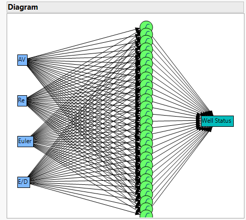
The independent variables are AV, Re, Eu, and ε/D. The dependent variable is well status. Well status is used to identify whether the fractured well is “clean” or “not clean”?
The model prediction was evaluated using two statistical parameters (R2 and RASE). R2 is the coefficient of determination. It is a statistical measure in a regression model that determines the proportion of variance in the dependent variable that can be explained by the independent variable. Root Average Square Error (RASE) is a standard way to measure the error of a model in predicting quantitative data. RASE can be thought of as some kind of (normalized) distance between the vector of predicted values and the vector of observed values. A RASE of zero implies that the average equation fits practically all the training and validation data.
Neural Boosted Model Training and Validation
Table 2 depicts training and validation plots for all collected data used in the Permian. An R2 exceeding 99%
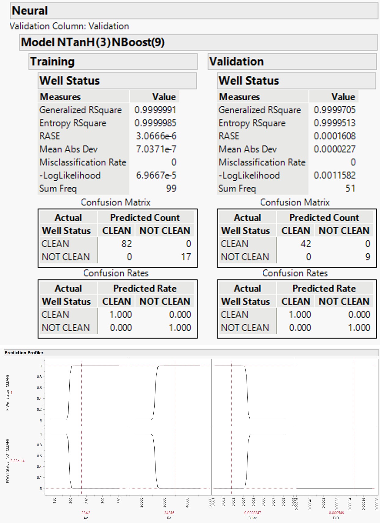
- was obtained for both training and validation. The R2 values replicate an excellent correlation. The RASE for testing and validation is practically zero. They are at 0.000006 and
- 0.000161 for testing and validation, respectively. In model testing 82 wells were recognized as “clean”, 17 were identified as “not clean”. In model validation, 42 were identified as
- “clean” and 9 as “not clean”.
Table 2: Neural trainisng and validation data.
Prediction profiler (Figure 2) proves that the well is totally “clean” for AV > 230, Re > 34,000, and Eu < 0.0028. The well is tagged as a “not clean” for AV < 200, R_e < 29,000, and _Eu > 0.0030.
Other Predictive Tools
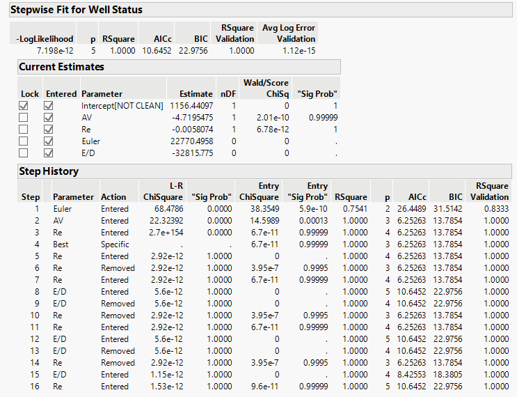
Stepwise fit: The stepwise fit for well status indicates that the coefficient of determination R2 = 1.0 (Table 3).
The Akaike’s Information Criterion corrected for small sample sizes (AICc) is a measure used in statistical modeling to assess the goodness of fit of a model while penalizing for the number of parameters in the model. It is particularly useful when dealing with a limited sample size. The AICc is defined as:
n AIC likelihood k c n k = +
( ) -2log 2 - -1
where:
( ) -2log likelihood is twice the negative log-likelihood of the model, k is the number of estimated parameters in the model, and
- n is the sample size.
- In the stepwise fit Table 3, ChiSquare for the intercept and the four independent variables, AV, Re, Eu, and ε/D was very close to zero, implying that the model can be taken as is and will not be reduced further, meaning that neither the intercept nor any of the four independent variables will be dropped nor disregarded from the empirical equation.
- The AICc for the developed WCC stepwise fit model is estimated at 10.6452 with an average log error validation that is close to zero (1.12 E-15). The developed empirical model formulation writes as follows:
- 1 156 - 4.720
- – 0.00581Re 22770
- - 32816 /
- WCC
- AV
- Eu
- D
- =
- +
Table 3: Stepwise fit for well status.
The AICc is an adjusted version of the Akaike Information Criterion (AIC) and is designed to account for potential bias in the AIC when the sample size is small relative to the number of parameters in the model. The penalty term n k n k increases as the number of parameters (k)
2 - -1 increases, but it is adjusted based on the sample size (n).
In general, when comparing different models, a lower AICc value indicates a better trade-off between model fit and complexity. Therefore, the model with the lowest AICc is often considered the preferred model among the candidates [39]. One reason that ( ) -2log likelihood is used is that the distribution of the difference between the full and reduced model ( ) -2log likelihood values is asymptotically ChiSquare. The degrees of freedom associated with this likelihood ratio test are equal to the difference between the numbers of parameters in the two models [40].
Researchers and analysts often use information criteria like AICc alongside other model comparison techniques, such as likelihood ratio tests, to make informed decisions about the most appropriate model for their data. In the regression model, BIC is defined as follows:
( ) ( ) -2log ln BIC likelihood k n = +
where k is the number of the estimated parameters and n is the number of observations used in the model.The BIC for the developed WCC stepwise fit model is estimated at 22.9756 and a ( ) -log likelihood close to zero (7.198 E-12). AICc and BIC serve similar purposes but have different penalties for model complexity. AICc is often preferred when dealing with smaller sample sizes, while BIC tends to favor simpler models, especially in larger datasets. Researchers may use both criteria and other model selection techniques to make informed decisions about the most appropriate model for their data (Burnham and [41].
Boosted Tree: In addition, boosting builds a predictive model in an additive manner. Instead of constructing a single complex model, it creates a sequence of simpler models (often decision trees) called layers. Each layer is trained sequentially. The training of a layer involves fitting a decision tree to the residuals (the differences between the observed and predicted values) of the model constructed from the previous layers. The purpose of fitting each layer based on residuals is to correct the errors made by the previous layers. Each subsequent layer focuses on the mistakes of the ensemble up to that point, improving the overall predictive accuracy. Typically, each decision tree in boosting consists of a small number of splits. These are often shallow trees, which helps prevent overfitting and ensures that each tree contributes a simple and focused correction. The training process involves minimizing the residuals, effectively refining the model’s predictions with each added layer. This process continues until a specified number of layers (or weak learners) are reached [42, 43, 44, 45].
In Table 4, the boosted tree for well status gave an R2 of 0.9974 and an RASE of 0.0026. The boosted decision tree technique used 152 layers on the 150 wells (with 99 training rows and 51 validation rows).The technique utilized 2 splits per tree with a learning rate of 0.073 and an overfit penalty of 0.0001, to evade overfitting of data.
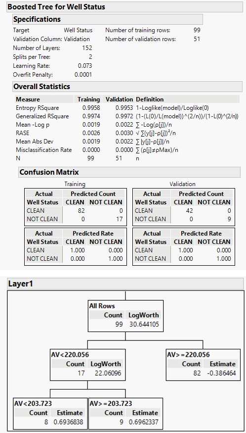
Figure 3 shows a decision tree (Layer 1) splitting, with 99 training rows. The splitting of 2 per tree is done on 17 training rows, where the fit based on residuals allows each layer to correct the fit for bad fitting from the previous layers. The final prediction for an observation is the sum of the predictions for that observation over all the layers.
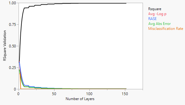
The R2 cumulative validation plot confirms that the RASE reduces to a minimum of 0.0026, with 152 layers. As a matter of fact, R2 converges of 1.00 as the number of layers increases and the probability misclassification rate is reduced to 0 (Figure 4). The misclassification rate acts as an important measure to decide the best model.
Decision Tree (Partition): The partition platform employs a recursive partitioning algorithm to build a decision tree. This means that the dataset is successively divided into subsets (partitions) based on the values of predictor variables.
The partitioning is done based on the relationship between predictor variables and the response variable. The algorithm identifies splits in the data that best predict, or explain the variation in the response variable. The partition algorithm explores all possible splits of predictor variables to find the ones that result in the best predictive performance. This involves evaluating different criteria or measures of impurity (e.g., Gini impurity, entropy) to determine the optimal way to partition the data at each step.
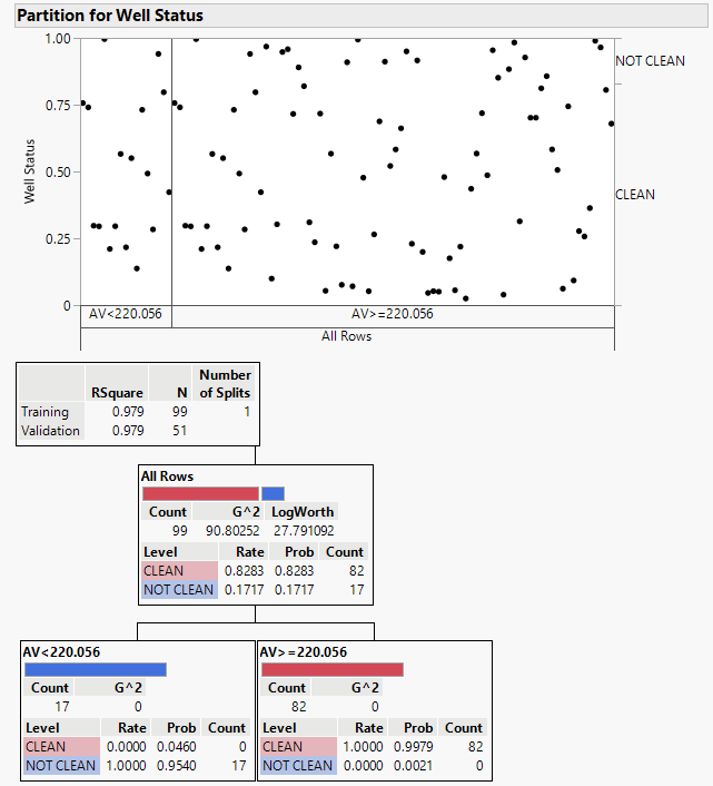
The splits or partitions are made recursively to form a tree structure. At each level of the tree, the algorithm decides on the best split, and the process is repeated for the resulting subsets until a stopping criterion is met. The final decision tree consists of a set of decision rules that guide the prediction of the response variable for new, unseen data. Each path from the root to a leaf node represents a combination of predictor variable conditions that lead to a specific prediction. The splitting process continues until a desired level of fit is reached or until a predefined stopping criterion is met. Stopping criteria may include a certain depth of the tree, a minimum number of data points in a leaf node, or other measures to prevent overfitting [42, 43, 44, 45]. The partition of well status graph indicates that for R2 for training (99 wells) is 0.979. That for validation (51 wells) is also 0.979. The partition graph also confirms that for AV <
220 wells are “not clean” and that for AV > 220 the wells are totally “clean” and defines a partition (a divide) at AV = 220.
Generalized regression Lasso: The generalized regression personality provides variable selection techniques, including shrinkage techniques such as the Lasso and Elastic Net.
The Lasso and Elastic Net are two popular techniques that perform variable selection as part of the modeling procedure. They are effective in handling situations with multicollinearity and high-dimensional data. Large datasets with many variables often exhibit multicollinearity issues. The presence of correlated predictors can lead to instability and poor performance in classical modeling techniques. The Lasso and Elastic Net address these challenges by performing variable selection and regularization. It accommodates continuous, binomial, count, or zero-inflated response variables. This flexibility makes it suitable for a wide range of modeling situations. The generalized regression personality is recommended for situations where users want to compare models obtained using different techniques. It allows for the fitting of models with various distributions and provides a basis for model comparison. This personality is recommended when there is an interest in variable selection, suspicion of collinearity in predictors, or a need to fit models for comparison with models obtained using other techniques.
In summary, the generalized regression personality is a versatile tool that addresses challenges associated with correlated and high-dimensional data. It is applicable to both large datasets with multicollinearity issues and small datasets, offering variable selection capabilities and flexibility in handling different response variable distributions. It is a valuable option for users seeking to build predictive models, reduce model complexity, or compare models across different scenarios [42, 43, 44, 45].
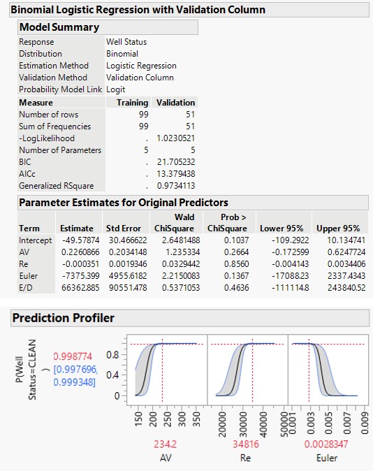
The binomial distribution was chosen because of set problem outcomes “clean” or “not clean”. The obtained generalized likelihood for a clean well is R2 of 0.97. The regression model used 5 parameters, an intercept and the 4 independent variables AV, Re, Eu, and ε/D. The following best fit equation was obtained:
-49.58 0.226 – 0.000351Re – 7357 66363 / WCC AV Eu D = + +
A ChiSquare value of 2.22 indicates that Eu is the independent variable with the highest predictive power. AV is the next powerful predictor.
The prediction profiler tool for the generalized regression model (Figure 6) confirms that the well is 99.9 % “clean” for AV ≥ 234, Re ≥ 34,816, and Eu ≤ 0.00283. The findings are in line with conclusions drawn from other predictive tools. K Nearest Neighbors: K Nearest Neighbors is a flexible and intuitive algorithm that makes predictions based on the proximity of data points in the feature space. Its nonparametric nature allows it to handle diverse datasets, but attention must be paid to predictor selection. The algorithm has found success in applications requiring classification or
However, for validation (black line, k=10), the misclassification rate is the lowest (0.196), the number of misclassifications is also the lowest, however, R2 the highest prediction tasks, such as image classification and medical diagnostics [42, 43, 44, 45].
The model selection plot (Figure 7) displays a solution path across k based on the misclassification rate for categorical response. The slider (red line) placed on the value of K=1 implies that model 1 is the best performing model for training (misclassification rate = 0.000, light grey line). Model 1 (marked with an asterisk) also has the lowest number of observations that are incorrectly predicted by the model.
with a value of 0.80981 (Table 6). That makes k=10 the best predictive model.
| Training | Validation | ||||||||
|---|---|---|---|---|---|---|---|---|---|
| K | Count | R2 | Misclassification Rate | Misclassifications | K | Count | R2 | Misclassification Rate | Misclassifications |
| 1 | 99 | 0.60245 | 0 | 0* | 1 | 51 | 0.54106 | 0.01961 | 1* |
| 2 | 99 | 0.75731 | 0.0101 | 1 | 2 | 51 | 0.63201 | 0.01961 | 1 |
| 3 | 99 | 0.80926 | 0.0101 | 1 | 3 | 51 | 0.65266 | 0.05882 | 3 |
| 4 | 99 | 0.8425 | 0.0101 | 1 | 4 | 51 | 0.65517 | 0.05882 | 3 |
| 5 | 99 | 0.85174 | 0.0101 | 1 | 5 | 51 | 0.70079 | 0.05882 | 3 |
| 6 | 99 | 0.84927 | 0.0202 | 2 | 6 | 51 | (0.72538 | 0.05882 | 3 |
| 7 | 99 | 0.84509 | 0.0202 | 2 | 7 | 51 | (0.73439 | 0.01961 | 1 |
| 8 | 99 | 0.85306 | 0.0202 | 2 | 8 | 51 | 0.73912 | 0.01961 | 1 |
| 9 | 99 | 0.83583, | 0.0202 | 2 | 9 | 51 | 0.80908 | 0.01961 | 1 |
| 10 | 99 | 0.84335, | 0.0404 | 4 | 10 | 51 | 0.80981 | 0.01961 | 1 |
Table 4: Misclassification rate comparison for 10 models.
In addition, the mosaic plot (Figure 8) proves that K = 1 model performs the best for training.
Furthermore, in the contingency figure (Figure 8), the mosaic plot is a graphical representation of the two-way frequency table (“clean” and “not clean”). A mosaic plot is divided into rectangles of varying dimensions; the vertical length of each rectangle is proportional to the proportions of the Y variable within each level of the X variable.
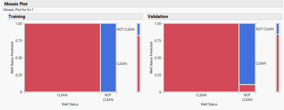
Figure 8: Mosaic plot for training Figure 8 a graphical representation that is designed to visually communicate the relationship and association between two variables (X and Y). X is “clean” or “not clean” and Y is the predicted probability. The width of partitions on the horizontal axis gives insight into the distribution of observations across different levels of the X variable. Meanwhile, the proportions and response probability on the vertical axis provide information about the relationship between the X and Y variables, including a reference to the null hypothesis of no association.
Table 7 summarizes all six predictive tools. The top 3 tools for training are Fit Stepwise (R2 = 1.0, RASE = 4.3 E-13), Nominal Logistic (R2 = 1.0, RASE = 5.8 E-12), and Neural Boosted (R2 = 1.0, RASE = 3.07 E-6). For validation, Fit Stepwise has an R2 of 1.0 and RASE of 6.4 E-14, Nominal Logistic has an R2 of 1.0 and RASE of 1.8 E-12, and Neural Boosted has an R2 of 1.0 and RASE = 0.00016.
| Training | ||||||
|---|---|---|---|---|---|---|
| Method | N | Sum Wgt | Entropy R2 | Misclassification Rate | RASE | Generalized R2 |
| Fit Stepwise | 99 | 99 | 1 | 0 | 4.30E-13 | 1 |
| Neural | 99 | 99 | 1 | 0 | 3.07E-06 | 1 |
| Boosted Tree | 99 | 99 | 0.9958 | 0 | 0.00262 | 0.9974 |
| Decision Tree | 99 | 99 | 0.9786 | 0 | 0.01916 | 0.9868 |
| Generalized Regression Lasso | 99 | 99 | 0.934 | 0 | 0.05773 | 0.9585 |
| K Nearest Neighbors | 99 | 99 | 0.6024 | 0 | - | - |
| Validation | ||||||
| Method | N | Sum Wgt | Entropy R2 | Misclassification Rate | RASE | Generalized R2 |
| Fit Stepwise | 51 | 51 | 1 | 0 | 6.40E-14 | 1 |
| Neural | 51 | 51 | 1 | 0 | 0.00016 | 1 |
| Boosted Tree | 51 | 51 | 0.9953 | 0 | 0.00297 | 0.9972 |
| Decision Tree | 51 | 51 | 0.9785 | 0 | 0.01942 | 0.9869 |
| Generalized Regression Lasso | 51 | 51 | 0.9308 | 0.0196 | 0.08954 | 0.9565 |
| K Nearest Neighbors | 51 | 51 | 0.5411 | 0.0196 | - | - |
Table 5: Summary table for training and validation using the 6 predictive tools.
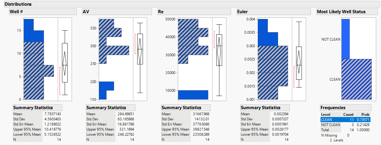
Using the developed code (see Appendix) for the Spraberry wells, 14 wells (“clean” and “not clean”) from Woodford have been used to test the validity of the code. 3 wells have been identified as “not clean” since AV is lower than 200, Re is less than 10,000, and Eu is larger than 0.003 (Figure 9).
JSL allows JMP users to write scripts, enabling the recreation of analysis results. Power users often use JSL to extend JMP’s functionality and automate analyses in production settings. JSL in JMP serves as a powerful scripting language that allows users to automate analyses, extend functionality, and reproduce results. It is particularly useful for documenting and automating repetitive tasks, making it a valuable tool for data analysis and exploration in JMP [42, 43, 44, 45].Top of Form The JSL code is depicted in the paper Appendix. In the future, an interface will be developed to create a user-friendly software that will be commercialized.
Commercializing the JSL Code
The commercialization of the developed JSL code involves several steps to ensure that the software is sold or distributed in a way that aligns with the business goals and legal requirements. The following is an outline of a general guide that will help with the commercialization of the JSL code:
Code licensing: Choose a suitable software license that aligns with the business goals. Common licenses include open-source licenses like MIT, GPL, or commercial licenses. These licenses will allow retaining more control over the code. Intellectual Property Protection: Consider protecting intellectual property through patents, trademarks, or copyrights, depending on the nature of the code and the type of protection it requires. Documentation Creation: Develop comprehensive documentation that explains how to install, configure, and use the JSL code. This will be crucial for users and potential customers to understand the product. User Interface Building: The code has a user interface that is user-friendly and visually appealing. A well-designed interface can enhance the overall user experience. Licensing Mechanisms Implementation: Licensing mechanisms are implemented to control access and usage. This includes activation keys, license files, or other methods to verify the legitimacy of users. Strategy Pricing: A pricing strategy for the software will be decided. This is a one-time purchase, subscription-based, or a combination of both. Distribution Channel Set Up: Distribution of the software will be through a website, third-party platforms, or a combination of both. In addition, aligning the distribution channels with the business strategy will be ensured. Processing Payment: To handle transactions, a secure and reliable payment processing system will be set up. This might involve integrating with third-party payment processors or using an e-commerce platform. Marketing and Sales: To promote the software, a marketing strategy will be developed. This may involve creating a website, utilizing social media, and reaching out to potential customers. Besides, offering demos or free trials, to attract users, will be considered. Customer Support: A system will be established to provide customer support. This will include email support, forums, or a dedicated support team. We will guarantee good customer support to maintain customer satisfaction. Staying Compliant: We will ensure that the commercialization efforts comply with all relevant laws and regulations. This will include data protection laws, export regulations, and other industry-specific requirements. Regular Updates and Maintenance: We will commit to maintaining and updating the software to fix bugs, add new features, and ensure compatibility with the latest technologies.
This was a general guide, and the specific steps that will be taken will depend on the nature of the JSL code, the target market, and the business goals. Besides, legal professionals will be consulted to ensure that all legal and regulatory requirements are met.
Conclusion
Six Predictive tools have been used to further validate the developed WCC correlations for 151 Spraberry formation fractured wellbores from West Texas. The Neural Boosted model showed an excellent degree of fit with an R2 of 1.0000 for training and an R2 of 1.000 for validation. The strong correlation between WCC and the annular velocity, Reynolds, and the Euler Numbers have been tested with 14 wells from the Woodford formation in Oklahoma.
A JSL code has also been written to identify whether fractured wellbores are “clean” or “not clean” from debris and bridge plug fragments. The input used are annular velocity, Reynolds, and Euler Numbers. It was proved that for AV > 220, Re > 29,000, and Eu < 0.003 fractured wellbores are all 99.99% deemed “clean”. The code will allow operators to identify conditions for which completed fractures wells are “clean” of debris and fragments of bridge plugs.
A commercialization document has been established to emphasize that the software is properly marketed and complies with legal considerations.
References
-
Kalogirou S (2003) Artificial Intelligence for the Modeling and Control of Combustion Processes: A Review. Progress in Energy and Combustion Science 29(6): 515-566.
-
Babikir HA, Abd Elaziz M, Elsheikh AH, Showaib EA, Elhadary M, et al. (2019) Noise Prediction of Axial Piston Pump Based on Different Valve Materials using a Modified Artificial Neural Network Model. Alexandria Engineering Journal 58(3): 1077-1087.
-
Shahab M (2000) Virtual Intelligence Applications in Petroleum Engineering: Part 1-Artificial Neural Networks. Journal of Petroleum Technology 52(9): 64- 73.
-
Cevik A, Sezer EA, Cabalar AF, Gokceoglu C (2011) Modeling of the Uniaxial Compressive Strength of Some Clay-bearing Rocks using Neural Network. Applied Soft Computing 11(2): 2587-2594.
-
Graves A, Liwicki M, Fernandez S, Bertolami R, Bunke H, et al. (2009) A Novel Connectionist System for Unconstrained Handwriting Recognition. IEEE Transactions on Pattern 31(5): 855-868.
-
Lippman RP (1987) An Introduction to Computing with Neural Nets. IEEE ASSP Magazine 4(2): 4-22.
-
Ali JK (1994) Neural Networks: A New Tool for the Petroleum Industry. European Petroleum Computer Conference, UK.
-
Rispler K, McNichol J, Matiasz K, Rheinlander M (2001) Using an Artificial Neural Network to Develop a Wall- Loss Model for Coiled Tubing Fracturing Operations. SPE/ICoTA Coiled Tubing Roundtable, Texas, USA.
-
Ahmadi MA (2016) Toward a Reliable Model for Prediction of Drilling Fluid Density at Wellbore Conditions: A LSSVM Model. Neurocomputing 211: 143- 149.
-
Rolon L, Mohaghegh SD, Ameri S, Gaskari R, McDaniel B (2009) Using Artificial Neural Networks to Generate Synthetic Well Logs. Journal of Natural Gas Science and Engineering 1(4-5): 118-133.
-
Tariq Z, Elkatatny S, Mahmoud M, Ali AZ, Abdulraheem A (2017) A New Technique to Develop Rock Strength Correlation Using Artificial Intelligence Tools. SPE Reservoir Characterization and Simulation Conference and Exhibition, UAE.
-
Elkatatny S, Mahmoud M, Tariq Z, Abdulraheem A (2017) New Insights into the Prediction of Heterogeneous Carbonate Reservoir Permeability from Well Logs Using Artificial Intelligence Network. Neural Computing and Applications 30(9): 2673-2683.
-
Mousa T, Elkatatny SM, Mahmoud MA, Abdulraheem A (2018) Development of New Permeability Formulation from Well Log Data Using Artificial Intelligence Approaches. Journal of Energy Resources Technology 140(7): 072903.
-
Alsabaa A, Gamal H, Elkatatny S, Abdulraheem A (2021) New Correlations for Better Monitoring the All-oil Mud Rheology by Employing Artificial Neural Networks. Flow Meas Instrum 78(6): 101914.
-
Ren X, Hou J, Song S, Liu Y, Chen D, et al. (2019) Lithology Identification Using Well Logs: A Method by Integrating Artificial Neural Networks and Sedimentary Patterns. Journal of Petroleum Science and Engineering 182(5): 106336.
-
Ahmed AS, Mahmoud AA, Elkatatny S, Mahmoud M, Abdulraheem A (2019) Prediction of Pore and Fracture Pressures Using Support Vector Machine. International Petroleum Technology Conference, China.
-
Abdelgawad K, Elkatatny, Moussa S, Mahmoud M, Patil S (2018) Real-Time Determination of Rheological Properties of Spud Drilling Fluids Using a Hybrid Artificial Intelligence Technique. Journal of Energy Resources Technology 141(3): 1-9.
-
Mahmoud AA, Elkatatny S, Abdulraheem A, Mahmoud M (2017a) Application of Artificial Intelligence Techniques in Estimating Oil Recovery Factor for Water Drive Sandy Reservoirs. SPE Kuwait Oil & Gas Show and Conference, Kuwait.
-
Mahmoud AA, Elkatatny S, Abdulraheem A, Mahmoud M, Ibrahim O, et al. (2017b) New Technique to Determine the Total Organic Carbon Based on Well Logs Using Artificial Neural Network (White Box). SPE Kingdom of Saudi Arabia Annual Technical Symposium and Exhibition, Saudi Arabia.
-
Elkatatny S, Al-AbdulJabbar A, Mahmoud AA (2019) New Robust Model to Estimate the Formation Tops in Real-Time Using Artificial Neural Networks (ANN). Petrophysics 60(6): 825-837.
-
Al-Abdul-Jabbar A, Elkatatny S, Mahmoud M, Abdulraheem A (2018) Predicting Rate of Penetration Using Artificial Intelligence Techniques. SPE Kingdom of Saudi Arabia Annual Technical Symposium and Exhibition, Saudhi Arabia.
-
Al-Abdul-Jabbar A, Gamal H, Elkatatny S (2020) Application of Artificial Neural Network to Predict the Rate of Penetration for S-shape Well Profile. Arab J Geosci 13: 784.
-
Gamal H, Elkatatny S, Abdulraheem A (2020) Rock Drillability Intelligent Prediction for a Complex Lithology Using Artificial Neural Network. Abu Dhabi International Petroleum Exhibition & Conference, UAE.
-
Mahmoud AA, Elkatatny S, Abdulraheem A, Mahmoud M, Ibrahim O, et al. (2017b) New Technique to Determine the Total Organic Carbon Based on Well Logs Using Artificial Neural Network (White Box). SPE Kingdom of Saudi Arabia Annual Technical Symposium and Exhibition, Saudi Arabia.
-
Mahmoud AA, Elkatatny S, Mahmoud M, Abouelresh M, Abdulraheem A, et al. (2017c) Determination of the Total Organic Carbon (TOC) Based on Conventional Well Logs Using an Artificial Neural Network. International Journal of Coal Geology 179: 72-80.
-
Mahmoud AA, Elkatatny S, Ali A, Abouelresh M, Abdulraheem A (2019b) New Robust Model to Evaluate the Total Organic Carbon Using Fuzzy Logic. SPE Kuwait Oil & Gas Show and Conference, Kuwait.
-
Mahmoud AA, Elkatatny S, Al-Shehri D (2020b) Application of Machine Learning in Evaluation of the Static Young’s Modulus for Sandstone Formations. Sustainability 12(5): 1880.
-
Mahmoud AA, Elkatatny S, Ali A, Moussa T (2019c) Estimation of Static Young’s Modulus for Sandstone Formation Using Artificial Neural Networks. Energies 12(11): 2125.
-
Tariq Z, Elkatatny S, Mahmoud M, Abdulraheem A (2016) A Holistic Approach to Develop New Rigorous Empirical Correlation for Static Young’s Modulus. Abu Dhabi International Petroleum Exhibition & Conference, UAE.
-
Elkatatny S, Mahmoud M, Mohamed I, Abdulraheem A (2018a) Development of a New Correlation to Determine the Static Young’s Modulus. Journal of Petroleum Exploration and Production Technology 8(1): 17-30.
-
Tariq Z, Elkatatny S, Mahmoud M, Ali AZ, Abdulraheem A (2017) A New Approach to Predict Failure Parameters of Carbonate Rocks Using Artificial Intelligence Tools. SPE Kingdom of Saudi Arabia Annual Technical Symposium and Exhibition, Saudi Arabia.
-
Gowda A, Elkatatny S, Gamal H (2012) Unconfined Compressive Strength (UCS) Prediction in Real-time While Drilling Using Artificial Intelligence Tools. Neural Comput Appl 33(13): 8043-8054.
-
Alsaihati A, Elkatatny S, Mahmoud AA, Abdulraheem A (2020) Use of Machine Learning and Data Analytics to Detect Downhole Abnormalities While Drilling Horizontal Wells, With Real Case Study. Journal of Energy Resources Technology 143(4): 043201.
-
Arehart RA (1990) Drill-bit Diagnosis with Neural Networks. SPE Computer Applications 2(4): 24-28.
-
Elkatatny SM (2017) Real-Time Prediction of Rheological Parameters of KCl Water-based Drilling Fluid Using Artificial Neural Networks. Arabian Journal of Science and Engineering 42(4): 1655-1665.
-
Alsabaa A, Gamal H, Elkatatny S, Abdulraheem A (2020) Real-Time Prediction of Rheological Properties of Invert Emulsion Mud Using Adaptive Neuro-fuzzy Inference System. Sensors 20(6): 1669.
-
Elkatatny S, Tariq Z, Mahmoud M (2016) Real-time Prediction of Drilling Fluid Rheological Properties Using Artificial Neural Networks Visible Mathematical Model. Journal of Petroleum Science and Engineering 146: 1202-1210.
-
Gamal H, Abdelaal A, Alsaihati A, Elkatatny S, Abdulraheem A (2021) Artificial Neural Network Model for Predicting the Equivalent Circulating Density from Drilling Parameters. 55th US Rock Mechanics/ Geomechanics Symposium, USA.
-
Akaike H (1974) A New Look at the Statistical Model Identification. IEEE Transactions on Automatic Control AC 19(6): 716-723.
-
Wilks SS (1938) The Large-Sample Distribution of the Likelihood Ratio for Testing Composite Hypotheses. Annals of Mathematical Statistics 9(1): 60- 62.
-
Burnham KP, Anderson DR (2004) Multimodel Inference: Understanding AIC and BIC in Model Selection. Sociological Methods and Research 33(2): 261-304.
-
JMP, Boosted Tree, Fit Many Layers of Trees, Each Based on the Previous Layer.
-
JMP, Partition Models, Use Decision Trees to Explore and Model Your Data help.
-
JMP, Generalized Regression Models, Build Models Using Variable Selection Techniques.
-
JMP, K Nearest Neighbors, Predict Response Values Using Nearby Observations.
- Nigeria’s Vulnerability in the Face of Global Energy Policy
- A Simulation Study of Investigation of Optimum Oil Production Performance by Applying Various Gas Injection Methods in Oil Reservoir
- Characterization of Permo-Triassic Reservoirs through Thermal Maturity Assessment of Westphalian Source Rocks in the Cheshire Basin
- Influence of Microwax on the Rheological and Thermal Behaviour of a Wax Crude Oil
- Real-Time Monitoring and Performance Optimization of Steam Injection in Heavy Oil Reservoirs Using Fiber Optic Sensing and Integrated Predictive Simulation Models
- Rapid On-Site Determination of the Total Petroleum Hydrocarbon Content of Soils by Handheld Fourier Transform Near-Infrared Spectroscopy: Development of a Global, Site- and Scanner- Independent Calibration Model