Accurate Oil and Gas Production Decline Curve Fit Using Cumulative Production-Production Rate- Time Linearized Form of Arp’s Hyperbolic Decline Equation

Nwankwo KO¹* and Nwankwo PC²

¹Chevron Nigeria Limited, Nigeria ²University of Ibadan, Nigeria

other methods.

Keywords: Oil and Gas Production; Cumulative Production; Hyperbolic Decline Equation

Introduction

Decline Curve Analysis is the practice of mimicking production trending as a function of time as exploitation Conceptual Article progresses. The strength of a decline curve tool lies in its ability to fit the decline trend, forecast with great measure of accuracy, the future trend and estimates reserves. Arps decline curve is as of now the most popular form of decline largely because it fits into this trend. Arps JJ [1] developed Decline curve empirically by principles of lost ratio. The Exponential, Hyperbolic and Harmonic declines were developed, also, by Arps JJ [2] in a later publication. Of these three declines, only hyperbolic decline does not have a direct linear form from Production rate and time equation. Exponential and Harmonic form of the rate trend with time could easily be transformed to straight line forms based on simple Algebraic operations [3].

Fetkovich MJ [4], came up with exact method of fitting Hyperbolic Decline curves by type curve matching4. These he did with discreet points of decline exponents. The major limitation is that it does not determine the unique decline exponent for any given Decline trend. It is however presently relied upon as one of the best methods for estimating decline exponent. Li and Horne, in 2005, published a linear form of the hyperbolic decline but its application was limited to diagnostic of the decline exponent and linking Fetkovich’s type curve to the derived linear form. Model was not used to determine decline constant and Initial Production Rate. Hence the linear form could not be used to fit the hyperbolic trend of even a smooth data much less a scattered data [5].

There has been no straight-line form documented in the literatures of Decline curve analyses that fit the Arp’s hyperbolic decline curve profile on production data without non-linear regression. This point is further underscored by the fact that there are a lot of programs and subroutines that fit hyperbolic decline profiles, and none exists for either exponential or harmonic decline profiles. Nwankwo KO, et al. [6], published two linear forms of the Arp’s hyperbolic decline equation namely the Rate-Rate Derivative-Time linear form and Decline Constant Harmonized linear form which best trended smooth data and scattered data respectively with an added iterative Initial rate program using error minimization method.

The aim of this paper is to establish a linear form of Arp’s Hyperbolic decline equation that can be used to explicitly fit the decline profile (without determining iteration on initial production rate). This will simplify the hyperbolic decline fitting, reduce computer time, and eliminate errors due to approximations. Furthermore, it would provide a unique linear form whose extrapolate is a natural fit and a perfect representation of the hyperbolic profile over the decline trend.

Arps Decline Curve

Arps JJ presented the generalized form of decline as a production rate function [1].

b q q bDt = + (1)

i

1 1 ( ) Where the constants: qi: Initial Production rate D: Decline constant B: Decline exponent He, also, classified Decline curves into three types [2]: Exponential (Constant percentage) Decline (b=0) [2]:

b q q bDt = + (1)

i

1 1 ( ) Harmonic Decline (b=1) [2] :

iq q Dt = +

(1b)

1 It is easily observed from either binomial approximation of equations (1) and (1b) and maclaurin series approximation that when Dt is far less than 1, ( ) 1 i q q Dt = − (1c)

Linear Forms of ARPS Decline Equations

The linear forms used to evaluate the constants in Arps Decline equation are:

Cum-Rate-Time Method

This was derived from the Cumulative Production, Production rate and time. This is based on principle that the ratio of remaining mobile fluid to instantaneous production is in partial linear variation with time. At any point, the remaining mobile fluid is calculated by subtracting the cumulative production from the initial mobile fluid volume (Maximum mobile fluid volume).

The hyperbolic decline equation, from equation (1), is given by, b q q bDt = +

i

1 1 ( ) Cumulative Production for Decline curve is given by Arps JJ [2]

t p N qdt ∆ = ∫

0 (3) Substituting, the hyperbolic decline curve equation (equation (1)) above into (3) and integrating gives, − +   ∆ = − +   − −   (4) i i b p q q N bDt D b D b

1 1 1 1 1 ( ) ( ) ( )

The term abs Q (Maximum Mobile fluid volume - i.e. Mobile fluid volume at time Zero) is expressed as:

i abs q Q D b = −

(5) (1 ) Subtracting equations (7) from (8) and dividing by flow rate equation (1) gives:

abs p Q N bt q D b b −∆ = + − −

( ) ( ) 1 1 1

(6) ( ) 1 1 P abs q b N Q qt D b b ⇒∆ = − − − −

(7a) P q qt abs N m q m qt Q ∆ = + + (7b) Where

1 qt b m b = −

(7b (i)) And

( ) 1 1 q m D b = −

(7b (ii)) Equation (7b) is a spatial linear equation and plotting p N ∆ against q and qt will give a straight line in a spatial co- ordinate system from which qi b and D could be obtained.

However, the hyperbolic fit could also be obtained by method of multiple linear regression using equation 7(a). This will calculate the exact hyperbolic parameters, qi b and D from which the equation will be obtained. This can easily be done by representing the above equation in the form Furthermore, the decline constant, D, and decline exponent, b, are obtained from equation (7c) as m b m = − qt (7c (i))

1 qt

1 qt m D m

− = (7c (ii)) q Alternatively, abs Q could either be calculated from multiple regression analysis method in the appendix or be obtained graphically by plotting as the Z-intercept of the graph p N ∆ of against q and qt.

The decline constant, D, and decline exponent, b, are then obtained from equation (6) by plotting planar linear function.

abs p Q N bt q D b b −∆ = + − −

( ) ( ) 1 1 1

(6) Introducing a Cumulative-rate transform variable, η , as abs p Q N

q η −∆ = (8a) ( ) ( ) 1 1 1 b t D b b η ⇒ = + − −

(8b) Equation (8b) is a singularity (indeterminate) in the case of a harmonic equation (b=1) but fit exists in exponential case (b=0).

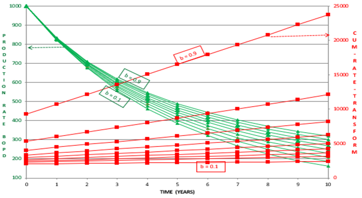
A plot of η against t will give a straight line as shown in Figure 1 (family of hyperbolic decline curve and their respective cum-rate-time transform plot), from which b and D could be calculated deterministically from the slope and intercept using the equations below:

1 Slope b Slope = +

(8b(i))

1 Slope D Intercept + =

(8b(ii))

Click to enlarge

Scattered Data

Real production data are not often smooth. However, this linear formulation gives a good fit on scattered data with defined decline trend. In cases where this formulation cannot fit Arp hyperbolic profile on the production data, we may smoothen the curve using the method in” improved decline curve fit using as in Decline Constant Harmonization method. From equation (1c) we for different data set, n, we obtain equation (9) below.

( ) ( ) 1 in in n q q D t t = − − (9)

Likewise, the Cumulative production profile can be smoothened. This involves fitting the quadratic curve approximation in equation (4) above to give equation (10) on cumulative production within a short period. This approximation is derived from binomial expansion of the second term of equation (10) to the third term (neglecting the fourth term upwards) fits all hyperbolic decline profile.

− +   ∆ = − + −   − −  

1 1 1 1 1 in b i i p n q q N bD t t D b D b ( ) ( ) ( ) ( )

(10) Yields the equation below by quadratic approximation of the binomial expansion:

( ) ( ) 2 2 in in p in n n D N q t t t t   ∆ = − − −     (11)

Maclaurin expansion of the second term in equation (10) (considering (t - tn) as variable and truncating at the third term) also yields same result. The resulting periodic decline, in D , will then be tested for geometrical attenuation and if no geometric relationship is observed, the Decline constant is then be harmonized as done in the rate - time fit with the equation below.

n b n b in p p D nt D bDt Dr

+   −      = + =    

1 1 ( ) ( )

(12) ( ) n in p D nt Dr ⇒ = (13)

The Decline constant trend ensuring a geometric attenuation pertain is derived and used to smoothen data for Production rate and cumulative production. This trend preserves the hyperbolic nature of the data trend while smoothening the cumulative and production rate trend with time. It should be noted that the real data (production data I and II-Tables 1 & 2 and Figures 2-4) that were used to validate this linear form did not utilize data smoothening but gave an excellent trend. Most importantly check the Appendix for the multiple regression equations used to solve this production data I and II problems.

Click to enlarge

Click to enlarge

Click to enlarge

Conclusion and Recommendation

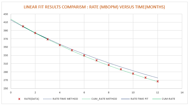
Cum-rate-time method of fitting hyperbolic curves is always the best method and most accurate when rate- time data is smoothened. Although a reduction in time intervals can also improve rate time method but it’s never as accurate as cum-rate-time method. As mentioned above, the cumulative production-time data is naturally smoothened to improve the accuracy of the fit. This method estimates qi, b and D and this underscores the reason for its accuracy. The three recommended methods for this fit are the graphical (A three - dimensional graph plot), least square method and the combined least square and two-dimensional graph. The least square method is the most solvable while the three - dimensional graphical is the simplest but will require some graphical software aid.

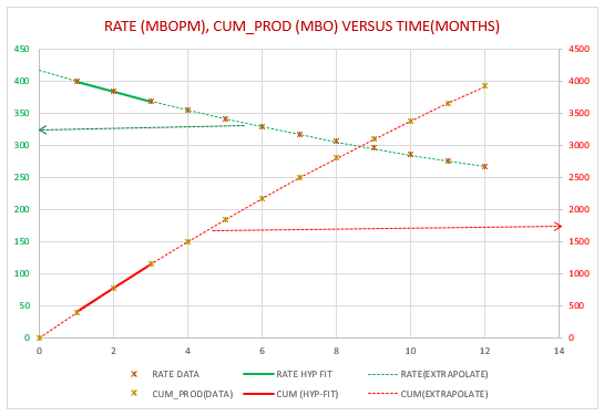
Calculation of Mobile oil in place is enabled from the cum-rate-time linear fit methodology and this is simply the Z-intercept of the straight line fit in the three-dimensional graph. This is one important value that has not been realized from decline curve fit since principles has been formulated from the principles of loss ratio. The Cumulative Production - Production Rate - Time fit is a near perfect fit of cumulative production, production rate versus time and hence accurately trends production rate as a function of time. Based on the trended rates over time a 5-year reliable forecast is achievable with production rate with time assuming production conditions remain same.

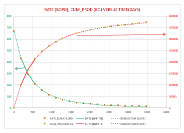
In likewise manner, the cumulative production trends over time are even more accurate than the production rate time profile. A 7-year reliable forecast of cumulative production versus time can be obtained. This was demonstrated in Figure 4 above. The usefulness of this trend cannot be overemphasized. Based on fluency of the Cumulative production trend with time, the estimation of remaining reserves at any point in time (which is a direct subtraction of the cumulative production at that point in time from the Recoverable oil (expected total recovery at abandonment)) is obtainable. This makes reserves accounting very flexible and trending the reserves with time is also fluent.

Booking of reserves entails using the two methods, Production rate versus time and Production rate versus Cumulative production profile methods. A comparison of results from both methodologies is done and sometimes plots of reserves estimated are done to get the point of similar results which is the reserves value that will be booked. These are no longer necessary with this linear form as the reserves will be deterministic and no longer iterative. Most wells are without totalizers to measure their production. Cumulative production of wells and hence cumulative production of the associated reservoirs from such wells are complex estimating and the results from such are not accurate. However, using this method and building a solution node network the different wells cumulative production calculation accuracy can be improved upon.

References

-
Arps JJ (1945) Analysis of Decline Curves. Transactions of the AIME 160(1): 228-247.
Arps JJ (1956) Estimation of Primary Reserves. Transactions of the AIME 207(1): 24-33.
Liu F, Mendel JM, Nejad AM (2009) Forecasting Injector/ Producer Relationships from Production and Injection rates Using an Extended Kalman Filter. SPE Journal 14(4): 653-664.
Fetkovich MJ (1980) Decline Curve Analysis Using Type Curves. Journal of Petroleum Technology 32(6): 1065- 1077.
Mead HN (1956) Modifications to Decline Curve Analysis. Transactions of the AIME 207(1): 11-16.
Nwankwo KO, Nwankwo PC (2020) Improved Oil and Gas Production Decline Curve Fit Using Rate - Time Linearized Form of Hyperbolic Decline. International Journal of Science and Engineering research 11(3): 1670-1678.
- Nigeria’s Vulnerability in the Face of Global Energy Policy
- A Simulation Study of Investigation of Optimum Oil Production Performance by Applying Various Gas Injection Methods in Oil Reservoir
- Characterization of Permo-Triassic Reservoirs through Thermal Maturity Assessment of Westphalian Source Rocks in the Cheshire Basin
- Influence of Microwax on the Rheological and Thermal Behaviour of a Wax Crude Oil
- Real-Time Monitoring and Performance Optimization of Steam Injection in Heavy Oil Reservoirs Using Fiber Optic Sensing and Integrated Predictive Simulation Models
- Rapid On-Site Determination of the Total Petroleum Hydrocarbon Content of Soils by Handheld Fourier Transform Near-Infrared Spectroscopy: Development of a Global, Site- and Scanner- Independent Calibration Model