Automated Segmentation of Optic Disc and Cup in Color Fundus Images
An automatic Optic disc and Optic cup detection technique which is an important step in developing systems for computer-aided eye disease diagnosis is presented in this paper. This paper presents an algorithm for localization and segmentation of optic disc from digital retinal images. OD localization is achieved by circular Hough transform using morphological preprocessing and segmentation is achieved by watershed transformation. Optic cup segmentation is achieved by marker controlled watershed transformation. The optic disc to cup ratio (CDR) is calculated which is an important parameter for glaucoma diagnosis. The presented algorithm is evaluated against publically available DRIVE dataset. The presented methodology achieved 88% average sensitivity and 80% average overlap. The average CDR detected is 0.1983.
Vijay M Mane* and Rahul Bal
Vishwakarma Institute of Technology, Pune, Maharashtra, India
Maharashtra, India, Tel: 9822550134; Email: manevijaym@gmail.com detected is 0.1983.
Keywords: Image processing; retina; optic disc; optic cup; glaucoma
Introduction
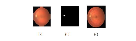
An optic disc (OD) is one of the most important structures of human retina [1] and their detection is an important step in computer aided diagnosis of various eye diseases [2]. In color fundus image, OD appears as a round bright yellowish or white region having shape more or less circular as shown in Figure 1. Optic cup plays an important role in glaucoma detection [3], the enlargement of which with respect to OD is an indicator of glaucoma.
![Figure 1: Optic cup plays an important role in glaucoma detection [3], the enlargement of which with respect to OD is an indicator of glaucoma.](/fulltextimages/3234/fig_1.jpeg)
Literature Review
Chaum, et al. [1] proposed a method based on Bayesian classifier to extract OD. By obtaining confidence image map, the point with highest value represents OD center. Cook, et al. [2] proposed a method based on intensity variation as OD has higher intensity variation than other regions in the retina image. Jin, et al. [3] proposed a method to locate OD based on mathematical morphology. Grisan, et al. [4] located OD region based on optimization technique. Convergence point of blood vessels is identified as OD center. Ghalwash, et al. [5] Detected OD using matched directional filters.
Rinton, et al. [6] proposed a genetic algorithm to detect OD boundary. Tegolo, et al. [7] proposed regression based method to find OD boundary. Barmanb, et al. [8] used morphological approach to segment OD. Ginneken, et al. [9] Segmented OD based on point distribution model by using optimized cost function. Basu, et al. [10]
proposed a method based on correlation filter to segment OD. Methodology
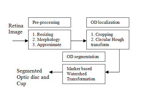
The OD localization and segmentation is implemented as shown in Figure 2.
Pre-processing
The input RGB image is resized by factor 0.2 while keeping the aspect ratio as that of original image. The green channel is selected for processing as red channel is more saturated and blue channel has low contrast. The Mathematical morphology in image processing is utilized which is a non-linear methodology that is suitable for analyzing shapes in the image. A closing operation is performed on the resized green channel image using Structuring Element (SE) followed by an opening operation. The closing operation performs dilation followed by erosion while opening operation performs erosion followed by dilation. The formulations for implementing dilation and erosion are as follows in equation 1 and 2. Dilation: C(x,y)= Maximum {A(x-i,y-j) * B(i,j)} (1) Erosion: C(x,y)= Minimum {A(x-i,y-j) * B(i,j)} (2) Where A(x,y) is the input image and C(x,y) is the resulting image obtained after A(x,y) has been processed with a m*n template B(i,j). B is called the structuring element where
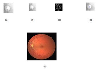
0 ≤ i ≤ m-1, 0 ≤ j ≤ n-1 The closing operation with octagonal SE of size 6 pixels is performed in order to fill the vessels in which dilation removes blood vessels and then erosion restores the boundaries. The size of SE is selected such that it keeps actual OD edge and removes all vascular structures on OD region. After performing the closing operation, an opening is performed to remove large picks. The image reconstruction is then performed on an opened image as shown in Figure 3a. The approximate OD center is obtained after thresholding the reconstructed image as shown in Figure 3b and 3c.
Circular Hough Transform
The hough transform is used for finding any shape which can be represented by a set of parameters. A circle can be transformed into a set of three parameters, representing its center and radius, so that the Hough space becomes three dimensional. A circular shape is described by parametric equation as defined in equation 3.
$$ (\mathrm {x} - \mathrm {p}) 2 + (\mathrm {y} - \mathrm {q}) 2 = \mathrm {z} 2 (3) $$ Where (p,q) is center of circle of radius z that passes through (x,y). The following steps are involved in procedure: 1) An accumulator space is created first which is made up of a cell for each pixel, initially setting all of these values to zero. 2) For every edge point in image (x,y),all cells are incremented, according to the above equation which could be center of circle. These cells are represented by ‘p’ in above equation. 3) All possible values of ‘q’ are found for all possible values of ‘p’ found in previous step. 4) The cells having the highest probability of being the location of the required circle are searched. These are those cells whose value is greater than its neighborhood cells.
An Accumulator space has peaks where circles obtained from each edge point overlap at centers of any circles detected. The maximum accumulator value is then found out which corresponds to radius that matches the OD and corresponding center is detected as OD center. The intermediate steps output is shown in Figure 4 (a-e) for OD localization.
OD Segmentation using Watershed Transformation
The image is considered as topographic surface where the altitudes are the gray level of the image is considered in the watershed transformation. The region edges correspond to high watersheds and low gradient regions correspond to catchment basins which are homogeneous. The watersheds are defined as the lines separating these catchment basins, which belong to different minima. The regions that the watershed separates are called catchment basins.
The watershed lines represent the boundaries of the objects if each local minimum corresponds to an object of interest under consideration. The watershed may results into many small regions when it infers catchment basins from gradient of the image. To avoid this condition, we used marker controlled watershed transformation in the presented approach. Here two markers are defined- (a) Internal marker, and (b) External marker. The catchment basins are generated by these markers in final segmentation.
In the presented approach, internal marker is selected as a circle having its center and radius is at center and 0.92 times that of radius obtained using circular Hough transform respectively as shown in Figure 5a. While external marker is selected as a circle as shown in Figure 5b with same point as a center as that of internal marker and having radius 1.2 times that of radius obtained using circular Hough transform so that it covers foreground region.
The factor is selected as 1.2 to maintain the distance between two markers. The Gradient of the image is calculated as the input to watershed transformation. We have used gradient magnitude as segmentation function. The Watershed of imposed markers with gradient of image provides the contour of the OD.
The OC segmentation is performed using morphology and watershed transformation. The marker controlled watershed transformation is applied to filtered image to segment OC. As grey level variation is very high in cup area, it is first removed by morphological closing. Then watershed transformation is applied to morphological gradient as shown in Figure 5g of median filtered image by considering locus of OC, k(m,n) that has been calculated as internal marker and square containing OC as external marker centered at (m,n) followed by imposed markers on gradient image produces cup boundary as shown in Figure 5h. The cup to disc ratio (CDR) is also calculated to detect glaucoma.
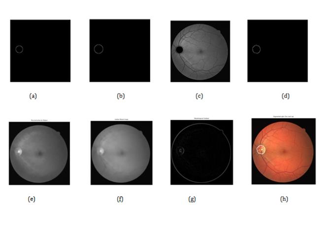
Figure 5: Optic disc (OD) and Optic cup (OC) segmentation: (a) internal marker for OD segmentation as circle considering OD center obtained using CHT in previous step as center and radius as 0.92* Q (Q as radius obtained using CHT), (b) external marker for OD segmentation as circle considering CHT processed center and radius as 1.2*Q, (c) marker controlled watershed transformed image which superimposes internal and external markers on gradient (sobel operated gradient) of original image, (d)OD boundary (watershed line), (e) Reconstructed image (reconstruction by dilation) for OC segmentation, (f) median filtered image, (g) morphological gradient of median filtered image, and (h) final segmented result of OD and OC (OC segmentation using marker controlled watershed transformation).
Experimental Results
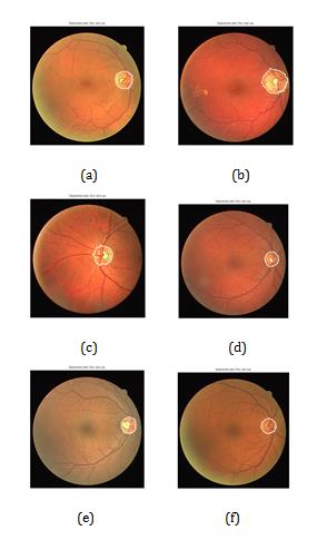
The experimentation of the proposed method has been done using standard DRIVE (Digital Retinal Images for Vessel Extraction) database [11]. The sample output is as shown in Figure 6. We validate the presented methodology using ground truth that was manually set by the experts on the images. In order to analyze the performance of algorithm the ratio R and sensitivity are calculated.
| Image | Sensitivity | R | CDR | ||||||||
|---|---|---|---|---|---|---|---|---|---|---|---|
| 1_test | 0.97509 | 0.90861 | 0.20736 | ||||||||
| 4_test | 0.94366 | 0.97953 | 0.10035 | ||||||||
| 5_test | 0.93004 | 0.83647 | 0.03855 | ||||||||
| 6_test | 0.8983 | 0.9179 | 0.2887 | ||||||||
| 7_test | 0.86153 | 0.85823 | 0.19275 | ||||||||
| 8_test | 0.99818 | 0.44963 | 0.22939 | ||||||||
| 9_test | 0.96853 | 0.81724 | 0.09575 | ||||||||
| 10_test | 0.83956 | 0.83846 | 0.23309 | ||||||||
| 11_test | 0.85346 | 0.83192 | 0.38117 | ||||||||
| 12_test | 0.99169 | 0.94192 | 0.30244 | ||||||||
| 14_test | 0.82721 | 0.80456 | 0.25934 | ||||||||
| 15_test | 0.62958 | 0.62406 | 0.2675 | ||||||||
| 16_test | 0.94684 | 0.8881 | 0.22287 | ||||||||
| 17_test | 0.92953 | 0.89537 | 0.17667 | ||||||||
| 18_test | 0.95189 | 0.79356 | 0.16426 | ||||||||
| 20_test | 0.94563 | 0.91342 | 0.13459 | ||||||||
| 22_training | 0.81423 | 0.73987 | 0.25374 | ||||||||
| 24_training | 0.87474 | 0.80733 | 0.23373 | ||||||||
| 25_training | 0.79493 | 0.79059 | 0.11835 | ||||||||
| 26_training | 0.98208 | 0.60934 | 0.00986 | ||||||||
| 27_training | 0.84488 | 0.76606 | 0.17765 | ||||||||
| 28_training | 0.94535 | 0.85651 | 0.13574 | ||||||||
| 29_training | 0.74089 | 0.73846 | 0.16516 | ||||||||
| 31_training | 0.95801 | 0.55927 | 0.09781 | ||||||||
| 32_training | 0.6101 | 0.59591 | 0.29814 | ||||||||
| 33_training | 0.59389 | 0.56347 | 0.33698 | ||||||||
| 34_training | 0.95507 | 0.84053 | 0.20556 | ||||||||
| 35_training | 0.88384 | 0.86231 | 0.11668 | ||||||||
| 36_training | 0.92102 | 0.87549 | 0.19215 | ||||||||
| 37_training | 0.91834 | 0.89974 | 0.20488 | ||||||||
| 38_training | 0.91585 | 0.88791 | 0.20488 | ||||||||
| 39_training | 0.90129 | 0.88397 | 0.2691 | ||||||||
| 40_training | 0.83943 | 0.83267 | 0.22961 | ||||||||
| Average | 0.8783273 | 0.800259 | 0.198331 |
Table 1: Performance measures of proposed method with respect to ground truth. Column 1: Image label; Column 2: Sensitivity; Colu
= Area G D Area D R GU
Where G is the ground truth and D is the detected circle.
Where TP (True positive) and FN (False negative), TP is number of OD pixels correctly classified and FN is number of OD pixels that were not detected. The CDR which is the ratio of number of pixels in optic cup to number of pixels in optic disc is also calculated. This parameter is used for the glaucoma analysis [12]. The Glaucoma is present in the image if CDR exceeds 0.3 value. We found glaucoma in two cases.
The algorithm is applied on 33 images for evaluating the method. The results for these images are listed in Table 1. The presented methodology achieved 88% average sensitivity and 80% average overlap. The average CDR detected is 0.1983.
Conclusion and Discussion
An automatic system for detection of both optic disc and optic cup has been presented. The presented method uses combination of circular Hough transform using morphological preprocessing and watershed transformation to locate and segment OD respectively. The results presented here may further improved by improving preprocessing which provides approximate OD center. We used mathematical morphology to locate approximate OD center which causes a false detection in abnormal cases.
References
-
Chaum E, Tobin KW, Priya Govindasamy V, Karnowski TP (2007) Detection of anatomic structures in human retinal imagery. IEEE Transactions on Medical imaging 26: 1729-1739.
-
Cook HL, Boyce JF, Sinthanayothin C (1999) Automated localization of optic disc, fovea and blood vessels from digital colour fundus images. British journal of ophthalmology 83(8): 902-910.
-
Park M, Jin JS, Luo S (2006) Locating the optic disc in retinal image. IEEE international conference on computer graphics, pp: 14-145.
-
Foracchia M, Grisan E, Ruggeri A (2004) Detection of optic disc in retinal images by means of geometrical model of vessel structure. IEEE Transactions on Medical imaging 23(10): 1189-1195.
-
Ghalwash AZ, Yousssif AA, Sabry AA, Abdel-Rahman Ghoneim (2008) Optic disc detection from normalized digital fundus image by means of vessels direction matched filter. IEEE Transactions on Medical imaging 27(1): 11-18.
-
Carmona EJ, Rincón M, García-Feijoó J, Martínez-de- la-Casa JM (2008) Identification of the optic nerve head with genetic algorithms. Artif Intell Med 43(3): 243-259.
-
Rosa LD, Tegolo D, Alina Lupascu C (2008) Automated detection of optic disc location in retinal images. 21st IEEE Symposium on computer based medical systems, Finland, pp: 17-22.
-
Niemeijer M, Abramoff MD, Ginneken BV (2007) Segmentation of Optic disc, macula and vascular arch in fundus photographs. IEEE Transactions on Medical imaging 26: 116-127.
-
Basu A, Ryder R, Lowell J, Hunter A, Steel D (2007) Optic nerve head segmentation. IEEE Transactions on Medical imaging 23(2): 256-264.
-
DRIVE: Digital Retinal Images for Vessel Extraction.
-
Joshi GD, Krishnadas SR, Sivaswamy J (2010) Optic disc and cup segmentation from monocular color retinal images for glaucoma assessment. IEEE Transactions on Medical imaging 30(6): 1192-1205.
- Origin, Evolution, and Functional Impact of Short Insertion- Deletion Variants in Human Genomes: A Review
- Harnessing Molecular Glues for Next-Generation Vaccine, Cancer and Cardiovascular Disease Drug Development: A Comprehensive Review
- Lateral Cervical Epidermal Inclusion Cyst in a Paediatric Patient: A Rare Case Report
- Malarial Plasmodium Falciparum with Hepatitis B and C Virus Infections among Blood Donors in Ife Central Local Government Area, Ile Ife, Osun State, Nigeria
- Withanolides and Withaferin A- What’s next in Ashwagandha Research
- Designing of Dual Pulse Photoacoustic Tomography for Imaging of Drug-Response and Tumor Growth