K-means Clustering Algorithm for Myocardial Infarction Classification
Heart attack is one of the main causes of death around the world. The electrocardiogram (ECG) is considered as an effective method to diagnose heart diseases. In this study, the classification approach will be applied to distinguish between myocardial infarctions (MI) subtypes. The abnormalities approval depends on morphological analysis used to detect the appearance or absence of some specific features in ECG graph. The classification approach consists of many basic steps such as data segmentation and various kinds of noise removal. Stemming filter will be used for detection of some features through a large number of data. Features selection and normalization approaches will be used for data validation and significant clustering. Finally, the K-means clustering will be used to differentiate between MI subtypes. The statistical analyses such as Precision, Recall, and F-Score were used to evaluate the performance of the K-mean algorithm. The F-score achievement is indicated at 0.98% in significant clustering and with 87.61% in right classification of MI subtypes.
Introduction
Myocardial infarctions (MI) are classified into ST elevation (STEMI) and non-ST elevation (NSTEMI) in accordance to the changes in the ECG graph [1]. ECG is considered as one of the most common diagnostic techniques used to evaluate the MI sub-class. By observing the cardiograph trace patterns, doctors can understand the state of the heart disease [2]. The baseline and shape of ECG graph help to evaluate the healthy functioning of the heart. Some features (morphological root) are used to determine the frequency and amplitude in ECG waveform. The increasing or decreasing in discrete time amplitude due to the diseases caused an appearance or disappearance of new segments in an ECG graph. Four (MI) subtypes (infero-postero-lateral (IPL); antroseptal (AS); infero-latera (IL); anterior (A)) will be studied and their leads are (L1; aVR; V1; V2; V3;V4; V5;V6)
Clustering and Classification
Clustering algorithm is used to group the data points without advance knowledge; oftentimes, clustering algorithm is used for forming a group of objects whose positions are accurately known. Classification is a mining technique used to predict group membership for data instances. Generally, several signal processing techniques and computer programming methods can be used for interpreting the heart disease. Some studies have discussed the topic, however, several challenges have been found during the automatic classification approach [3]. Few approaches of cardiograph classification methods into clinical practice were used, and the predictive capacity of these methods remains controversial and still inaccurate. Clustering technique, which is considered as a vector quantization, is used to quantify the ECG physical quantity in order to analyze and reduce a large number of data to a small number of features. The k-means clustering approach based on unsupervised machine learning has been applied. In general, ECG clustering is a complex process that requires many steps to achieve the final classification result. These steps start from signal segmentation, noise removal, feature extraction / selection, super vector construction, data weighting, clusters/centroids, and finally the classification approach. Features extraction phase include stemming filter, which is used for data reduction to a small number of features, such as wave shape or morphologic in discrete time amplitudes. Features must be strong enough to enhance its significance in the classification task. The process also includes normalization filter, which helps in the configuration of the training database. Finally, the K-mean classifier will be applied to differentiate between MI sub-classes, and the effectiveness on right decision making must be tested [4].
Statement of the Problem
Heart diseases are becoming the main significant reason for sudden death around the world [5]. Since 1970, many studies have deployed different mining approaches and computer programs that could assist the doctors in interpreting diseases according to the ECG graph shape [6]. Different classification algorithms can be used to differentiate between heart attack subtypes [7]. In this study, the classification approach is made according to American College of Cardiology Foundation (ACCF) [8] and software data mining techniques.
Material and Method
Participations & Data Collection
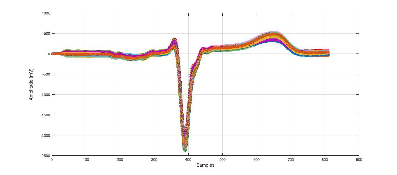
The ECG data is available online [9]. The database contains cardiology clinic data saved as standard text format, ECG lead I, recorded for 20 seconds, digitized at 500 Hz with 12-bit resolution over a nominal ±10 mV range. In this study, the data include normal ECG (healthy heart function) and four subtypes of myocardial infarction (MI). The data included 90 subjects (44 male, 46 female), four healthy subjects and 12 subjects with MI. The average age is between 13 and 75 years old. The dataset included eight leads [aVR; L1; V1; V2; V3; V4; V5; V6] in both normal and MI subtypes, each lead contained about 65,000 samples. This continues the time signals that will be discrete to pulses, and each separate pulse will contain 808 samples.
ECG Clustering and Classification Approach
The automatic algorithm method as shown in Figure 1 includes the following steps: Initial data collection and segmentation; Noise removal; R-wave detection; Matching phase; Stemming filter; Normalization; frequency distribution; k-clusters creation and Partitions (Voronoi diagram); centroid generation for each (k) clusters as the new mean. Afterwards, the k-means clustering algorithm will be applied for testing pulse to find the subtype where the pulse belongs to. The near means will be created for all centroids, and then the testing pulse will be assigned to one or more centroids according to the maximum value that will be found.
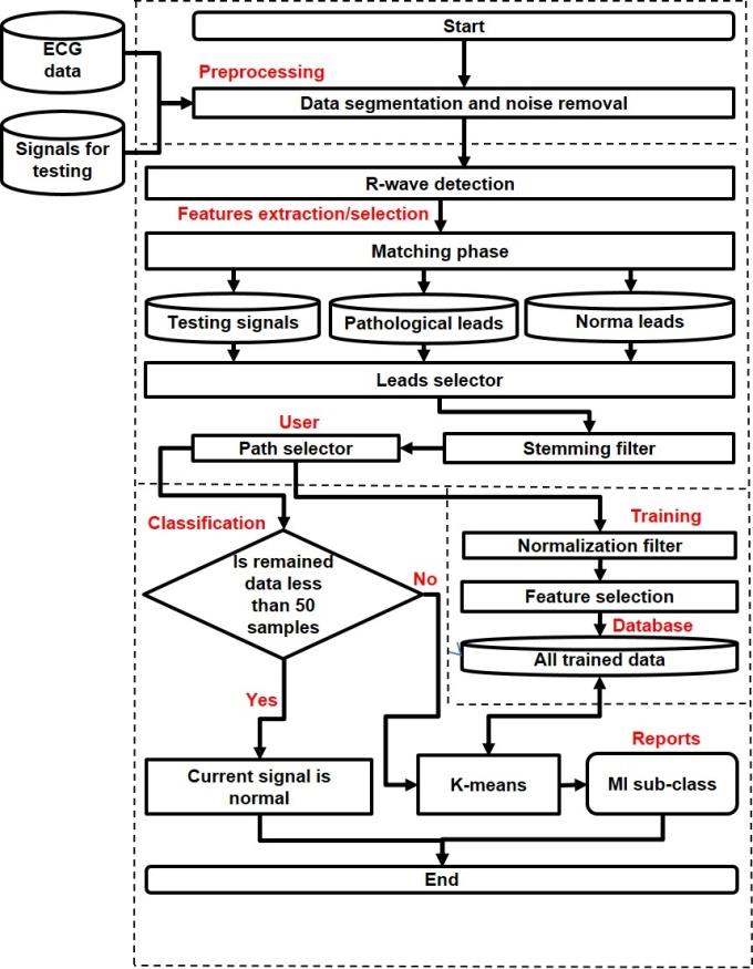
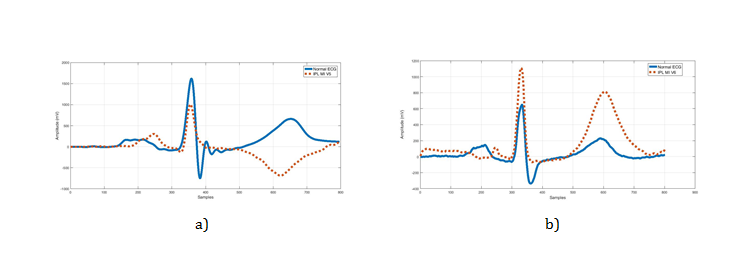
The K-mean cluster is considered as an unsupervised learning technique –which is used for exploratory data analysis that finds the hidden intrinsic structures or groupings in ECG data (morphological root). The morphologic root, as shown in Figure 2, shows a morphological variation between normal and abnormal ECG (the appearance of some segments different from normal signal).
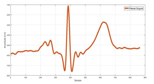
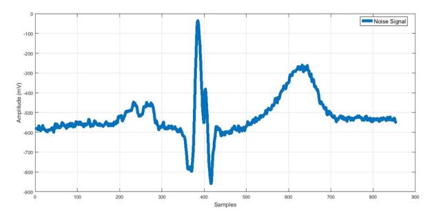
| Preprocessing impulse response (IIR)) [10]. The low-frequency noise can be removed with IIR low-pass filter [10], also linear Remove Artifact: Different sources of noise, which could trend can be de- trended using Notch filter [11] as shown appear in ECG signal, can be removed by using filtration in Figure 3. techniques such as digital filter from MATLAB® (Infinite | impulse response (IIR) | ) [10]. The low-frequency noise | |
| can be removed with IIR low-pass filter [10], also linear | |||
| Remove Artifact: Different sources of noise, which could | |||
| trend can be de- trended using Notch filter [11] as shown | |||
| appear in ECG signal, can be removed by using filtration | |||
| in Figure 3. | |||
| techniques such as digital filter from MATLAB® ( | Infinite |
a) b)
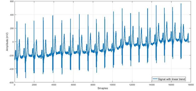
c) d) Figure 3: ECG waveform artifact and noise removal: a) Signal corrupted with motion artifacts from cardiology clinic database; b) Filtered signal after IIR low-pass filter; c) Signal with base line attenuation; d) De-trend signal after using Notch filter.
R-wave detection: For similarity comparison all MI data with Normal ECG, matching phase must be applied. The idea of matching lies behind the fact that after finding all R-wave (Figure 4), this peak sample will be reassembled in a new database. Wavelets analysis technique was used to detect the R peak value. Additionally, it was used to transform separate pulses into different frequency bands enabling a sparser representation of the signal [12]. The wavelets decompose signals into time-varying frequency components, because signal estimation can be easier when working with separate pulses representations (Figure 4).
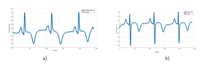
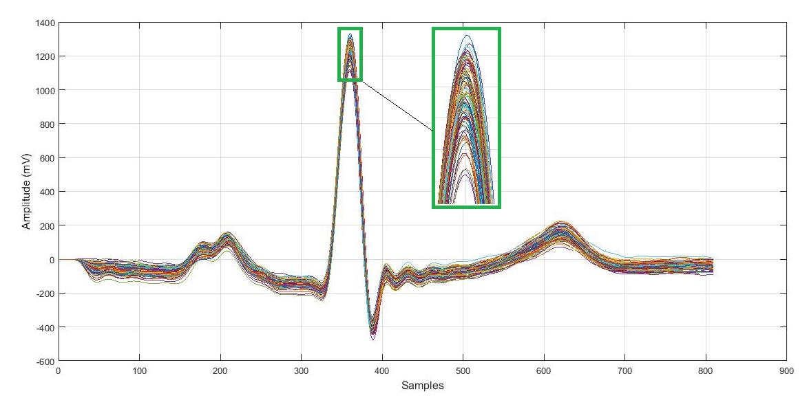
pulses must be matched in one raw. Therefore, the algorithm gathers all pulses in a new table based with the condition of unifying all R-waves in one raw (Figure 5).
Leads Selection
Feature extraction: Leads selection is an automatic program that is used to compare two selected leads, these leads must strongly belong to the same lead type. For example, if the recorded pathological signal came from V5 lead, the other normal lead must be V5 as well to compare with Figure 6. After that, the stemming filter for data reduction is applied. The remained data will contain segments of the pathological signal that indicate the differ part from the normal rhythm. Features extraction is an attempt to find strong morphological variation in diseases group that will monitor the diseases’ subtype. The stemming filter uses data reduction and the remaining data contain some segments from the signal that indicates the different part from the normal. Stemming filter is based on similarity function. Similarity function is used to compare all samples in pathological leads with the reference signal (the normal), all samples in the pathological group that share the same value with the normal will be removed. Remaining data contain morphological roots that have a property difference from normal leads (Figure 6).
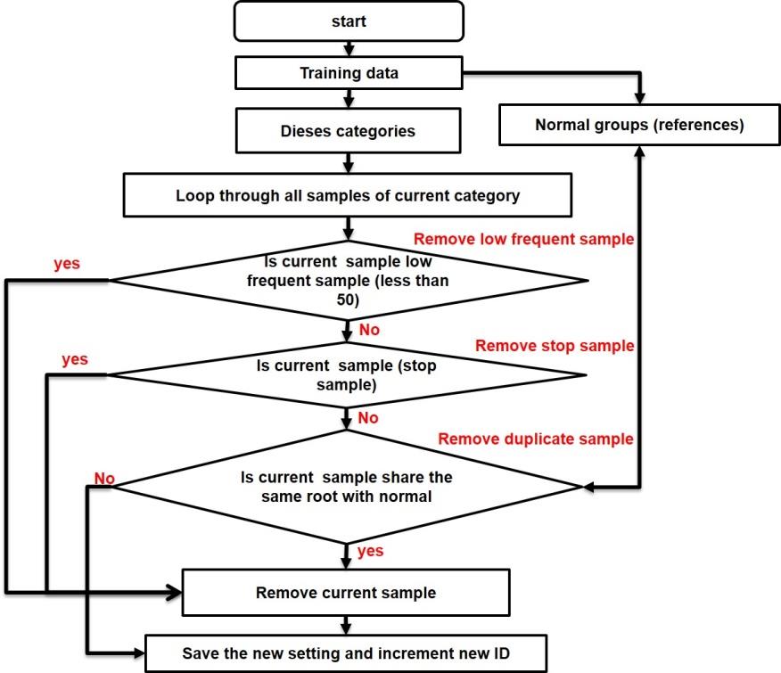
Many methods can be used for stemming task. The rule-based approach [13] could be suitable for (MI) classification task. Rule-based approach uses rules to make deductions, such as {IF 'condition' THEN 'result'}, and this looks like if the current sample is similar to the sample in normal category then delete this sample. The rule-based stemmer uses morphological analysis for feature generation; the features here look like finding the place in diseases cardiograph which is different from normal. The algorithm can be summarizing as followed (Figure 7):
- If current sample shares the same property with normal, then current sample will be removed.
- If current sample has low frequent through current set of data (less than 50), then current samples will be removed.
• If current sample is stop sample such as (spaces/alphabet/ Symbols …etc.), then current sample will be removed.
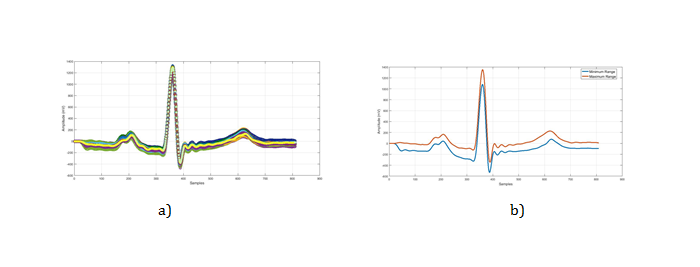
calculated in order to find the median level of the amplitudes. This range will be calculated only for the normal leads while diseases leads will remain the same.
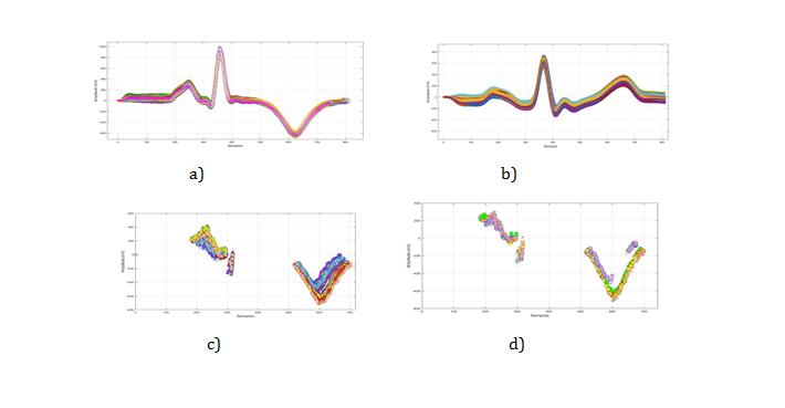
The next example demonstrates the stemming algorithm used to reduce the size and the density of the cluster (Figure 9). In the experiment, matched inferio- posterio-lateral- lead V5 was utilized. The result shows a perfect progress in data reduction when dealing with a highly complex signal such as ECG (Figure 9 (b)), which contains a huge number of samples that do not contribute in the classification task.
Data validation has been given much attention because the classification accuracy depends completely on the right feature selection, and also any mistakes during the training process will cause lack of classification in decision-making. Firstly, the normalization is used for eliminating encoding or missing input data to a single common character set. Secondly, the system must specify train data at their mean, and scales the unit standard deviation, thus, samples weighting technique must be applied in order to construct the super vector of (n) weighted samples for each groups; “normalized-formula” will be used for this task:
$$ = \frac {f _ {\mathrm {i K}} * \log \left(\frac {N}{n _ {i}}\right)}{\sqrt {v}} $$ N f n *log a iK i iK 2 ∑ M N f n = *log iK 1 j i , (1) Where:
• iK a – The weight of the sample (i) through the ECG
pulse (k);
• iK f – The frequency of sample (i) through the ECG pulse (k);
• N – The number of ECG pulses through current sample where accord;
- in – The ECG pulse frequency for current sample;
- M – The total number of samples in current ECG pulse. The method implements for “sample frequency weighting” which uses the following formula:
$$ a _ {\mathrm {i K}} = f _ {\mathrm {i K}}, \tag {2} $$
• iK a – The weight of the sample (i) through the ECG pulse (k);
• iK f – The period of time the sample (i) occur through the ECG pulse (k).
Features selection
After normalization, the data will be represented as a vector of (n) weighted samples. However, some high weighted samples may have been concentrated in some pulses without the other, and the system will consider them as very important samples due to its great repetition, but this will depreciate the accuracy of classification. Therefore, it is important to find a normal frequency distribution of sample frequent through the set. The frequency distribution method is a summary of how often each value occurs by grouping values together. There are multiple ways to calculate frequency distribution (count if Function and frequency function (Figure 10)).
Features selection approach will be based on two types of “frequencies” calculation, sample frequency versus pulse frequency and vice versa:
- Sample frequency versus pulses frequency (in the scope of the current pulse versus data set) – which means that the number of times when the sample occurs within the current pulse; tf (t,d) = ft,d. where (t) is the number of times that the sample occurs through the pulse (d).
- Pulse frequency versus current sample (in the scope of the set) – which means that the number of pulses in which the current sample occurs at least once is the scaled inverse fraction of the pulses that contain the sample, obtained by dividing the total number of samples by the number of pulses containing current sample, and then taking the logarithm of that quotient $$ i d f (t, d) = \log \frac {N}{\left| \{d \in D: t \in d \} \right|} $$ (3)
- N: the total number of pulses in current set N D =
- { : } d D t d ∈ ∈ : The number of pulses where the sample (t) occurs (i.e., ( , ) idf t d not equal to zero).
• If the sample is not in the set, this will lead to a division-by-zero. It is, therefore, common to adjust the denominator to1 { : } d D t d + ∈ ∈
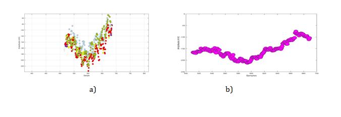
a) Anterior (V5) after stemming prosecedure. b) Anterior (V5) after normalization prosecedure. Pulse frequency method does not work with a small number of pulses in the set.
The K-Means Clustering
The model is used to assign a class label to diseases training data, for example, if X is a group of (n) rows, which correspond to observation, and the (K) is a column corresponding to a predictor, then the ECG pulse to certain category is considered as the final step of the classification process, in which the actual assignment of the ECG pulses to a certain predefined category is performed as shown in Table 1. In order to determine the mean value of the resulting data, the instance tf- idf weights vectors must be used for all ECG pulses in each category. The ECG pulse will be compared with all categories (centroids) in order to assign to a certain predefined group that is most similar.
For a better understanding of the principle of the classification process, the following summary of K-means clustering algorithm is defined: (iteration /cluster/ instance/dimensions):
1. Input K, set of points 1 2 ... x x
2. Place centroids 1... k c c at random locations 3. Find the nearest centroid for point and assign each point to cluster 4. Repeat 1 and 2 until convergence (iteration): For each point X1: o find nearest centroid c1, the Euclidean distance between instance xi and cluster centre cj, is given by D(xi,cj) o assign the point x1to cluster j For each cluster j=1...k:
o new centroid cj=mean of all points x1
o assigned to cluster j in the previous step: 1 ( ) ( ), ( ) 1... j j xi cj j c a
x a where a
$$ = \frac {1}{n _ {j}} \sum_ {x i \rightarrow c j} x _ {j} (a), w h e r e (a) = 1 \dots d $$ (4) o Stop when none of the cluster assignments changes.
Testing Random Pulse to a Certain Category
According to Figure 1, the user will be able to select the type of processing (path) for the purpose of classification. The testing data pass through the noise removal, R-wave detection and stemming process. Then the classifier will upload this testing data to the features space group as a new cluster, the space will be selected depending on the lead name of the testing signal. All samples of teasing data will be compared with the nearest neighbours centroid. The classifier will calculate (Formula 6) the total number of samples attached to each centroid, then gives these values in percentage.
Results and Discussion
Normal Category Training (the reference signal)
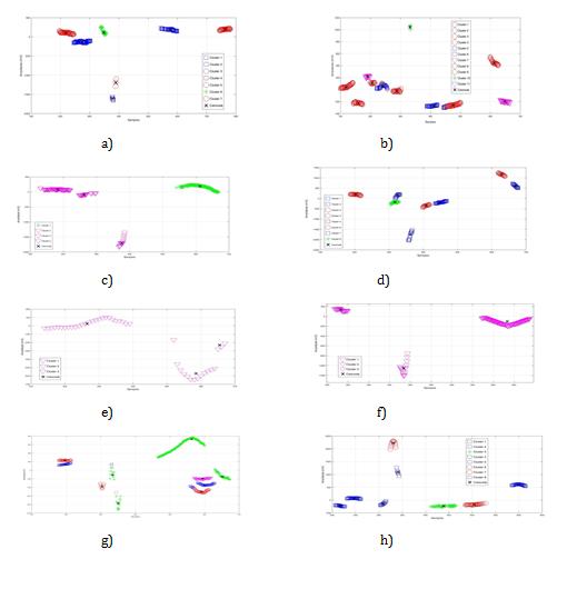
The normal category is used as a reference group (4 data set). Each row of (X) corresponds to one observation, and each column corresponds to one predictor (W). Each pulse will be represented as (n) weighted of features W (w1,…, wd), these features will be normalized in order to become clusters (k), then the (tf, idf) will be applied for leads centroids (AVR-L1-V1-V2-V3-V4-V5-V6) as in (Figure 11):
Pathological Data Training, MI Subtypes (groups)
Some medical evidence confirmed that some leads show the (MI) class better than the other leads [14]. The proposed algorithm for (IM) clustering is based on morphological variation of the ECG graph. First of all, stemming filter will be applied for all diseases data in order to remove duplicate and stop samples, remaining data will be normalized then will be considered as morphological changes which appear in ECG amplitude segments over the time series (Figure 12). The Morphological variation in each group will be assigned to the disease class, clusters will include (L1;aVR;V1;V2;V3;V4;V5;V6).
Testing Signals to Certain Category
The calculation of relevance testing signal with known lead to a certain category will be made as follows:
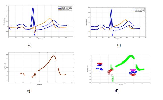
• If the total number of the remaining sample after stemming phase is less than 50, then current signal will be considered as a Normal; this is because when the testing signal is compared with normal leads, it will result to zero remaining data, because the stemmer will remove all samples in the test pulse due to 100% matching with normal group. Thus, if the total number of the remaining samples after stemming phase is over 50, then such signal will continue passing through the classification phases (normalization/weights vector, etc.).
• The classification process begins with the selection of one path to the new pulses in the features space (Voronoi diagram). For example, if the test signal is identified as V6 lead, then the path of the signal will be V6 feature space (Figure 13), in order to compare the distance between all samples in the test pulse with the nearest neighbours centroid (8 centroids).
• The matching coefficient of the test ECG signal will be assigned to a certain predefined category; the calculation in this case will be as a network flow problem (Points per-category or a tree diagram). The experiment results (Figure 13) show that 322 samples in the test pulse had nearest neighbours with "anteroseptal Lead (V5)". The calculation with formula (5) was used to find the matching coefficient, where (k) is the total number of samples which had similarity property with a predefined category (i), in a case by mean of "anteroseptal Lead (V5)".
$$A = \frac{K \in (i)}{\sum_{i=1}^{n}} \times 100$$
Where:
(A) - Matching coefficient,
(k) - Number of samples matchings with a certain predefined category (i),
($\sum_{i=1}^{n}$): The total number of samples on the current pulse.
Points Per-Category
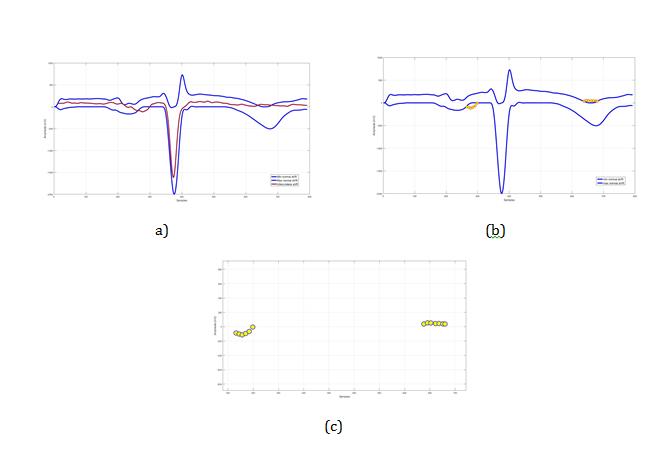
To illustrate the arrangement of the clusters of a test signals, the remaining nodes represent clusters (centroids) to where the testing data belongs to, the calculation will use formula (6). The test signal after stemming will appear as a separate segment (Figure 13c). On the other hand, trained clusters are grouped in the same way; therefore, it was necessary to configure a relationship taking into account the scattered centroids that belong to the same disease. The calculation is used to find matching coefficient, where the total number of samples in the testing category had similarity property to one or more predefined categories. The idea is that each M1 subtype may appear in different centroids, and to assign the disease subclass, the classifier must discover all these centroids and link them where they occur (Figure 13).
$$S = \sum_{i=1}^{n} 0^{(w_{ic} - a_{ik})}$$
where:
- S_Number of samples to Predefined category
- $w_{ic}$ - The weight (centroid) of the sample (i) which found in the new category of centroids (c) is the number calculated by the Classifier program and to be loaded from the (centroids XML-files);
- $a_{ik}$ - The weight of the sample (i) through the ECG pulse (k);
- $z$ - The number of samples frequent (i) which found through the centroid categories vector (c).
Once the calculation of the score table is completed for current ECG pulses, the system will calculate the max value of samples in the "Points per-category", the current pulse will be assigned to the category according to the max value that will be derived.
Classification Practices for Testing Signals to Certain Category
The next example shows a classification result of a testing signal chosen randomly from the cardiology clinic database. These signals with known lead number (V5) were not used in the training set. The number of samples that contains this signal is about (808 samples), 392 remained after stemming, 322 samples of them assigned to centroids (green star) which belong to anteroseptal subclass, each branch contains different leaf node. The class label decision will be taken after computing all samples that belong to different centroids (nodes). The decision label is assigned to anteroseptal acute infarction with 82.14% approximately according to nearest neighbors (by Euclidean distance) (Figure 13 and Table 1).
$$ A = \frac {3 2 2 \in a n t e r o s e p t a l}{3 9 2} * 1 0 0 = 8 2. 1 4 \% $$
| The total | ||||||||||||||||||||
|---|---|---|---|---|---|---|---|---|---|---|---|---|---|---|---|---|---|---|---|---|
| T o i | he total numbe | r d l | Mixing data | |||||||||||||||||
| Lead | number of | The total number of | Category | Matching | ||||||||||||||||
| f samples foun | between | |||||||||||||||||||
| number | samples after | samples to each centroids | name | coefficient % | ||||||||||||||||
| n current signa | centroids | |||||||||||||||||||
| stemming | ||||||||||||||||||||
| V5 | 808 | 392 | 0 | red circles = 33 | IL | 8.42% | ||||||||||||||
| green stars = 322 | AS | 82.14% | ||||||||||||||||||
| blue squares = 37 | IPL | 9.44% | ||||||||||||||||||
| tringle magenta = 0 | A | 0.00% |
Table 2: The P performance of k-mean Clustering for a VR lead.
Table1: Score table for a new testing signal to certain category.
Clustering Evaluation
Clustering approach is considered as an unsupervised learning method, the accuracy is not commonly used in unsupervised algorithms [15]. Thus, a different technique was used to evaluate the accuracy of the clusters.
ANOVA test
After the Stemming and Normalization steps, our work results showed several independent sets of data groups (Clusters). To determine whether these clusters are significantly different or not, we used the One-way Analysis of Variance (ANOVA) test. This test focuses on the mean of each cluster data -centroids- and compares them [16]. Thus compares the slopes regression lines. However, we report the results as significantly different depending on the probability value (P-value). P-value is historically based on random choice which is reasonably accepted choice. It states that if the P value is 0.05 or less, we conclude that the clusters are significantly different [17]. In that case, there is no point in comparing the intercepts. The intersection point of two lines is:
$$ X = \frac {I n t e r c e p t _ {1} - I n t e r c e p t _ {2}}{S l o p e _ {2} - S l o p e _ {1}} $$
1 2 (8)
2 1 $$ Y = I n t e r c e p t _ {1} + S l o p e _ {1} * X = I n t e r c e p t _ {2} + S l o p e _ {1} * X $$
| Best-fit values ± SE | Infero-Postero-Lateral | Infero-Lateral | Antroseptal | ||||||||
|---|---|---|---|---|---|---|---|---|---|---|---|
| Slope | 1.807 ± 0.1649 | -13.35 ± 0.307 | 0.5377 ± 0.129 | ||||||||
| Y-intercept | -450 ± 65 | 6572 ± 143.6 | -470.9 ± 56.87 | ||||||||
| X-intercept | 249 | 492.3 | 875.7 | ||||||||
| 1/slope | 0.5534 | -0.07492 | 1.86 | ||||||||
| Slope | 1.48 to 2.134 | -13.97 to -12.73 | 0.2764 to 0.7991 | ||||||||
| Y-intercept | -579 to -321 | 6283 to 6861 | -586.1 to -355.7 | ||||||||
| X-intercept | 209.1 to 281.4 | 488.6 to 496.2 | 733.3 to 1287 | ||||||||
| R square | 0.5506 | 0.9757 | 0.3196 | ||||||||
| Sy.x | 264.8 | 162 | 12.31 | ||||||||
| F | 120.1 | 1891 | 17.38 | ||||||||
| DFn, DFd | 1, 98 | 1, 47 | 1, 37 | ||||||||
| P value | <0.0001 | <0.0001 | 0.0002 | ||||||||
| Deviation from zero? | Significant | Significant | Significant | ||||||||
| Equation | Y = 1.807*X - 450 | Y = -13.35*X + 6572 | Y = 0.5377*X - 470.9 | ||||||||
| Number of X values | 614 | 529 | 464 | ||||||||
| Maximum number of Y replicates | 1 | 1 | 1 | ||||||||
| Total number of values | 100 | 49 | 39 | ||||||||
| Number of missing values | 514 | 480 | 425 |
Table 3: The P performance of k-mean Clustering for a VR lead.
As a result of the test, the P values are less than 0.05 for all the sub-classes (Table 2). That means the clusters are significantly different and there is no mixing data which could complicate the classification decision making task. We didn’t apply the test for the anterior sub-class in this example because it doesn’t appear in aVR lead.
We also used the Precision, Recall, and the F-Score for evaluating our clusters [18]. These scores were computed for every class pair (Table 3). Precision (P): Precision is the calculation of correct assigning points in dataset to the relevant class [19], by mean “How many of the points in each cluster is chosen correctly by the classified to be grouped in current cluster” (Table 3). The Precision is calculated as in equation 9.
Precision versus Recall and F-Score
The equation class name
$$ P \left(L _ {r}, S _ {i}\right) = \frac {n _ {r i}}{n _ {i}} $$
( , ) ri r i
(9) Where:
i rL - Class name with ( rn ) size iS - Class name with ( in ) size rn - The correct number of clusters results in - Number of all returned clusters results by the K-means Table3: Precision calculation.
Total Number of
Precision
Clusters ( in )
( , ) r i P L S
Lead L1 11 0.8900% Lead aVR 7 0.9300% Lead V1 3 1.0000% Lead V2 8 1.0000% Lead V3 3 1.0000% Lead V4 3 1.0000% Lead V5 10 1.0000% Lead V6 8 1.0000% Precision average 54 0.9775%
Recall (R): It is the fraction of actual objects identified. The number of correct results divided by the number of results that should have been returned [19]. The recall is calculated as:
$$ R \left(L _ {r}, S _ {i}\right) = \frac {n _ {r i}}{n _ {i}} [ 1 0 ] $$
( , ) ri r i
i $$ R \left(L _ {r}, S _ {i}\right) = \frac {5 2}{5 4} = 0. 9 6 2 \% $$
F-Score (F)
With an equal weight of Precision and Recall together gives a good combination called the F-Score [19]. It considers both the precision and the recall of the test to compute the score. The F-score can be interpreted as a weighted average of the precision and recall, where it’s best value at 1 and worst score at 0. It is calculated with the equation 11:
2* ( , )* ( , ) ( , ) ( , ) ( , )
$$ F \left(L _ {r}, S _ {i}\right) = \frac {2 * R \left(L _ {r} , S _ {i}\right) * P \left(L _ {r} , S _ {i}\right)}{R \left(L _ {r} , S _ {i}\right) + P \left(L _ {r} , S _ {i}\right)} $$ = 0.974% (11) r i r i r i r i r i
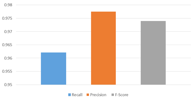
The F-score is considered as an average of the precision and recall, where reaches its best value at 1 (perfect precision and recall) and worst at 0. We achieved a value of F-score about 0.97% (Figure 14), achieved results prove that, stemming and normalization served in creating a great intergroup similarity and differentiate between the clusters.
Lead number
Remained data after
Number of samples attached to each centroids stemming
The Classifier Evaluation
The performance of the K-mean algorithm classification is compared with 10 cardiac clinical cases with four different MI subtypes (IL; IPL; AS; A). The accurcy of of the classifiation was 87% approximatly (Table 4).
Centroid assign to
Matching coefficient % Classifier accuracy
certain class red circles = 213 IL 81.60%
Others centroids = 48 --- 18.40%
Others centroids = 24 --- 12.70%
green stars =147 AS 92.50% Others centroids = 12 --- 7.50%
87.61% Others centroids = 93 --- 20.30%
| Others centroids = 37 | --- | 12.50% | |||
|---|---|---|---|---|---|
| V6 | 468 | blue squares = 374 | IPL | 80.00% | |
| Others centroids = 94 | --- | 20.00% | |||
| 156 | red circles = 149 | IL | 95.50% | ||
| Others centroids =7 | --- | 4.50% | |||
| V5 | 416 | blue squares = 351 | IPL | 84.00% | |
| Others centroids = 65 | --- | 16.00% | |||
| 410 | tringle magenta = 381 | A | 93.00% | ||
| Others centroids = 29 | --- | 17.00% | |||
| 337 | red circles = 321 | IL | 95.00% | ||
| Others centroids = 16 | --- | 5.00% |
Table 4: Classifier evaluation.
Conclusion and Future Work
Machine learning techniques used in medical diagnosis fields, such as classification and recognition systems, have improved to help medical experts in diagnosing attempt. This work presents unsupervised clustering algorithm used to differentiate between complexes ECG diseases subclass. Thus, good clustering method could produce a high inter-cluster similarity and low similarity between different clusters. The result shows that stemming filter is a quick and an accurate way to discover the morphology variation between disease MI subclasses. Our method helps in data reduction and clusters separation; stemming and normalization filters give a complete representation about the location of the disease morphology variation. In addition, major problems which could complicate the automation classification process had been resolved, and the achievement is evaluated with about 87.61% in right classification. The future work may involve using new clustering methods that could improve the performance of classifier in targeting other heart diseases, as well as increasing the flexibility of data entry, such as old electrocardiography sets and video capturing data.
Acknowledgement
The authors would like to extend their appreciation to the College of Applied Medical Sciences Research Center and the Dean of Scientific Research at Inaya Medical Colleges for funding this work.
References
-
The normal category is used as a reference group (4 data set). Each row of (X) corresponds to one observation, and each column corresponds to one predictor (W). Each pulse will be represented as (n) weighted of features W (w1,…, wd), these features will be normalized in order to become clusters (k), then the (tf, idf) will be applied for leads centroids (AVR-L1-V1-V2-V3-V4-V5-V6) as in (Figure 11): [INLINE_FIGURE:8:0] Figure 11: Matched normal ECG (V1).
- Origin, Evolution, and Functional Impact of Short Insertion- Deletion Variants in Human Genomes: A Review
- Harnessing Molecular Glues for Next-Generation Vaccine, Cancer and Cardiovascular Disease Drug Development: A Comprehensive Review
- Lateral Cervical Epidermal Inclusion Cyst in a Paediatric Patient: A Rare Case Report
- Malarial Plasmodium Falciparum with Hepatitis B and C Virus Infections among Blood Donors in Ife Central Local Government Area, Ile Ife, Osun State, Nigeria
- Withanolides and Withaferin A- What’s next in Ashwagandha Research
- Designing of Dual Pulse Photoacoustic Tomography for Imaging of Drug-Response and Tumor Growth