Growth-at-Risk: A Framework for Assessing Economic Vulnerability
The Growth-at-Risk (GaR) model estimates the probability that Gross Domestic Product (GDP) growth will fall below a specified threshold. Using the Quantile Regression approach, four Caribbean economies—The Bahamas, Barbados, Jamaica, and Trinidad and Tobago—were assessed to determine the impact of growth falling below the 2.0% threshold. For the subsequent three periods, growth remained above 2.0% in most forecasts. Additionally, an analysis specific to The Bahamas estimated the probability of GDP growth falling below 2.0%. The model was extended to simulate shocks and scenarios, and to calculate their effects on the likelihood that growth falls below the threshold. The results showed that growth usually exceeded the threshold in the forecasted periods.
Abbrevations
GaR: The Growth-at-Risk; GDP: Gross Domestic Product; VaR: Value-at-Risk; GARCH: Generalized Autoregressive Conditional Heteroskedasticity; NFCI: National Financial Conditions Index; FCI: Financial Conditions Index; GIV: Granular Instrumental Variables; IMF: International Monetary Fund; LDA: Linear Discriminant Analysis; SRI: Systemic Risk Indicator; MPI: Macroprudential Policy Indicator; CLI: Composite Leading Indicator; OLS: Ordinary Least Squares; RIR: Real Interest Rate; KDE: Kernel Density Estimation; BERT: Barbados Economic Recovery and Transformation.
Introduction
The concept of Growth at Risk (GaR) has emerged as a valuable tool in economic analysis, especially for assessing vulnerability to future downturns. GaR shifts focus from point forecasts of economic growth to the entire distribution of possible outcomes. It emphasizes the link between financial conditions and downside risks. Unlike traditional forecasts, GaR quantifies the probability and severity of potential negative growth scenarios. GaR also originated as an extension of value-at-risk (VaR) models. It estimates the expected distribution of GDP growth based on financial market conditions and other macroeconomic factors. Thus, GaR models link financial conditions with anticipated GDP growth to assess real-sector implications of systemic risk.
GaR offers policymakers valuable insights by enabling them to comprehensively assess economic risks. By quantifying the likelihood of downside scenarios, GaR helps them implement preemptive measures to mitigate potential downturns. Policymakers can use the framework in macroprudential policy to assess financial vulnerabilities and guide regulatory actions. Overall, GaR research advances economic analysis. By incorporating financial conditions and the entire growth distribution, GaR provides a more robust framework for assessing economic vulnerability and informing policy decisions.
This study examined three main approaches for multivariate GaR. First, copula-based models estimate marginal distributions using methods such as kernel density estimation. Researchers then select a copula function, such as the Gaussian or Clayton copula, to model the dependence structure of the variables. They use the joint distribution to simulate future scenarios for all variables. Second, GaR models with stochastic volatility capture dynamic interactions. These models track time-varying volatility using Generalized Autoregressive Conditional Heteroskedasticity (GARCH) and forecast future values for all variables, accounting for volatility changes. Thirdly, the quantile regression approach addresses the limitations of linear regression, by enabling researchers to explore how changes in macrofinancial conditions affect different quantiles of the GDP growth distribution.
With the GaR model, we seek to determine the probability that GDP growth will fall below a given threshold for four (4) Caribbean economies: The Bahamas, Barbados, Jamaica, and Trinidad and Tobago. We also extend the model to simulate macroeconomic shocks and scenarios, and then calculate their impact on the probability that growth falls below the threshold. Following the introduction, Section II investigates pertinent literature. Section III gives an overview of the selected countries’ economic performance. Section IV discusses the methodology and analyzes results. Section V summarizes the findings and concludes the paper.
Literature Review
The GaR Methodology was introduced by Tobias Adrian, Nina Boyarchenko, and Domenico Giannone in their 2019 paper, “Vulnerable Growth” [1, 2]. The paper models the entire distribution of future real GDP growth as a function of current financial and economic conditions and evaluates financial risks to economic growth in the United States. To assess economic and financial conditions, Adrian et al. used real GDP growth data from the Bureau of Economic Analysis and the National Financial Conditions Index (NFCI). The authors then employed semi-parametric quantile regressions to estimate the distribution. This approach describes the conditional relationship between future GDP growth and current financial and economic conditions. A skewed-t distribution was fitted to the quantile regression to smooth the results and derive a probability density function. The results indicated a nonlinear relationship between financial conditions and economic growth. The authors found that deteriorating financial conditions resulted in higher conditional volatility and a lower conditional mean of GDP growth. Adrian et al. also noted that upside growth risks were lower in most periods, while downside risks increased as financial conditions tightened. Measures of downside risk moved in line with financial conditions. Upside risk measures were more stable, meaning that lower quantiles depend more on current financial conditions for future GDP growth than upper quantiles. To verify these findings, Adrian et al. used both a fully parametric and a non-parametric approach. Both methods produced consistent results, confirming that the findings were robust and not dependent on their two- step method.
In an extension of the previous paper, Adrian, et al. [1] estimated the term structure of the predicted distribution of GDP growth for 11 advanced economies. The authors examined whether high GaR could occur in the near term due to loose financial conditions and whether it would be sustained. The panel quantile regression model used financial conditions, credit-to-GDP growth, the credit boom indicator, initial output growth, and inflation.
These variables helped derive the future distribution of GDP growth. Local projections were used to estimate the dynamic responses of GDP growth moments over 1 to 12 quarters. This allowed the authors to explore the progression of downside risk over time. Adrian et al. constructed a Financial Conditions Index (FCI) for each country in the panel. The FCI included up to 17 price-based variables, including short-term interbank risk spreads, corporate bond spreads, and stock return volatility. Estimates for the FCI were obtained using a vector autoregression model. This model varied over time due to changes in variable interactions and differences in data availability. The results showed that financial conditions had a greater effect on the lower fifth percentile of the growth distribution than on the median. This echoed a key finding in Vulnerable Growth. The term structure developed, showed that downside risks to growth are small in the near term with loose initial financial conditions, but increase in later quarters. When loose financial conditions combined with a credit boom, the authors noted a substantial adverse effect on the fifth percentile after quarter five, but no impact on the median. Adrian et al. also used the granular instrumental variables (GIV) approach to create a new instrument for financial conditions outside the FCI. This tested whether endogeneity bias between financial factors and GDP growth could explain their findings. The GIV results showed that the concern was unwarranted.
Since the introduction of the GaR approach, several authors have explored the concept in depth and evaluated its benefits for assessing growth risks. Further, policy institutions such as the International Monetary Fund (IMF)
have adopted the technique to monitor risks across countries. For example, Prasad [3] indicated that the GaR analysis was beneficial to policy-makers, as it could enhance their macro-financial surveillance activities. The reason is that the methodology focused on the entire growth distribution, which encompassed upside and downside risks to future economic growth, compared to the traditional point forecast used to guide policy decisions. Access to the complete distribution might encourage policy-makers to create and implement policies geared towards reducing risks to growth beforehand, compared to those that optimise outcomes under central scenarios [3, 4]. Further, it provided a framework for assessing the key drivers of future economic growth, which varied across the distribution of growth [5, 6, 7, 8, 9]. Lastly, the authors noted that GaR analysis could help gauge the impact of systemic risk on future GDP growth, thereby aiding the guidance and implementation of macro-prudential policies that protect financial stability and positively impact GaR [10, 12, 13, 14, 15, 16, 17, 18, 19, 20, 21]. However, Adrian, et al. [1] suggested that policy- makers might want to consider the inter-temporal trade- offs arising from their policy decisions, given their findings on the term structure of Growth-At-Risk. Moreover, when applying the GaR framework to country-specific data for risk measurement and macro-prudential policy implementation, a proper understanding of cross-country heterogeneity was needed, particularly for panel models. This was because a nation’s structural characteristics played an important role in shaping cross-country variations in GaR across risk indicators and time horizons [11].
Raluca [15] examined the potential impact of the GaR analysis on macro-prudential policy in Indonesia under different stress scenarios. The first step involved sorting 26 macro-financial variables into the categories of financial conditions (FINC), macrofinancial vulnerabilities (MAF), or other relevant factors (OTH), using factor analysis. The minimal residual method (MINRES) was used to determine which variables contributed most to the variability in the original series. Once determined, the author built a composite index for each partition, which was used to account for changes in financial conditions observed within each partition over time. This was followed by applying the quantile regression approach to the sample’s quarterly data, conditional on the partitions as mentioned above and a proxy for macroprudential policy. The GDP growth rate was included as a control variable. Findings showed that the materialisation of risk under three scenarios had significant benefits for improving the Growth-At-Risk contingent on the nature of their underlying vulnerabilities.
O’Brien, et al. [17] of the Central Bank of Ireland used the GaR framework to assess the likelihood and severity of future weak economic growth in Ireland, given current financial conditions and vulnerabilities. Results indicated that adverse growth outcomes in Ireland were most likely to occur during periods when threats to financial stability were rising. Further, near-term tail risks were heavily impacted by prevailing financial market conditions, while medium-horizon risks were more dependent on systemic financial vulnerabilities. The author’s analysis also suggested that structural features of Ireland’s economy increased the country’s susceptibility to weak growth outcomes.
Drenkovska, et al. [9], in a discussion paper published by the Bank of Slovenia, utilised the GaR approach to examine the connection between macro-financial conditions and economic activity in Slovenia. Following the three-step GaR procedure proposed by Prasad [3], the author developed, for analysis purposes, a financial conditions indicator (FCI) that aggregated metrics of financial stress and volatility from multiple financial markets. Moreover, the FCI included simpler metrics on yields and price indices that were regularly featured in policy debates or had been found to have good leading properties in other literature. In an effort to improve the quality of their regressions, the authors used Linear Discriminant Analysis (LDA) as a data reduction technique to extract common trends from relevant macro- financial events and remove idiosyncratic noise. Further, data reduction lowered the number of parameters needed for their estimations. Drenkovsak, et al. [9] also included the Domestic Systemic Risk Indicator (SRI) proposed by Lang, et al. [14] in their analysis, along with a macroprudential policy indicator (MPI) and a composite leading indicator (CLI). Results from the author’s baseline scenario supported the view that macro-financial conditions contained predictive signals of increased risks at the tails of the future GDP growth distribution. Further, estimates showed that the FCI represented downside risks to growth across all projection horizons.
At the same time, the SRI had the most significant adverse effects on the tail of the growth distribution around 8-12 quarters ahead. The negative coefficients on both indicators also indicated that higher systemic risk and financial stress are associated with lower GDP growth at the 10th percentile of the growth distribution, leading to lower growth forecasts for the distribution’s tail. In addition, the scenario analysis exercise showed that loose financial conditions were associated with sizeable leverage build-ups and higher short- term future growth. However, build-ups in leverage over time increased risks to medium-term growth in the Slovenian data; the same conclusion was reached by O’Brien, et al. [17] in Irish Data. Moreover, similar results from Lang, et al. [13] revealed that financial stress and vulnerability indicators contained information on growth-at-risk in the short term. In contrast, vulnerability indicators held information about GaR over the medium term [2, 9, 11, 12, 17]. Researchers also proposed modifications to the traditional growth-at-risk to improve the reliability and performance of GaR models, with a focus on assessing the impact of the COVID-19 pandemic on economic growth.
Chicana, et al. [8] modified the growth-at-risk framework by incorporating several model validation techniques to determine which forecasting density from their quantile regression results had the best predictive power for Peruvian data, adding a step to the methodology proposed by Prasad [3], which was used to build their GaR model. The authors utilised Schmidt, et al. [19] quantile-spacing approach to obtain a large sample of data from the estimated GDP growth quantiles, which were then fit to a broad set of probability distributions for interpolation. Findings indicated that macro-financial factors had heterogeneous effects on the distribution of future GDP growth across quantiles at different horizons.
Further, the negative impact of external financial conditions was more pronounced in the lower distribution quantile, consistent with the literature on GaR. After evaluating their models, the authors found that nonparametric density fitting via Kernel Density Estimation (KDE) and mixed normal density fitting produced the best density forecasts for Peruvian data. After establishing a reliable methodology for the GaR model, Chicana, et al. [8] proceeded with their counterfactual to evaluate the “Reactiva Peru” program sponsored by the government. The results of their estimations showed that the policy reduced the impact of the COVID-19 shock on the economy, as it would have had lower expected future growth and higher macro-financial risks if it had not been implemented [22, 23, 24, 25].
Mihail Yanchev [26] created an enhanced GaR Model, known as DeepGar, by proposing improvements to Adrian, et al. ’s [2] approach. The first enhancement consisted of generating quantiles simultaneously to alleviate the quantile-crossing problem. This was followed by introducing a quantile-crossing loss into the tilted loss function to prevent the above-mentioned problem further. Thirdly, the author used an artificial neural network implemented with the TensorFlow library to model non-linear relationships between the predictors and the target variable. The last change to the original procedure involved combining the above steps into a single model, which was optimised by minimising the tilted absolute loss and the least-squares loss. The author compared their deep-growth-at-risk model to a benchmark similar to Adrian, et al. [2] procedure and found that their proposed model outperformed the benchmark in predicting the adverse effects of the COVID-19 pandemic on GDP for the countries of interest (Bulgaria, Lithuania, Estonia, and Romania). It also performed better when modelling the recession caused by the unexpected shock of the global pandemic.
Overview of the Selected Countries Economic Performance
The Bahamas
The Bahamas has a service-based economy heavily dependent on two main sectors, tourism and financial services [7]. As a result, the economy is particularly vulnerable to external shocks, especially given that its tourists are primarily from the United States and that the financial services sector is heavily driven by foreign investment. Its vulnerability is evidenced by the sharp slowdown in growth following the 2008 global financial crisis to an average of 0.8 per cent between 2010 and 2019 [22]. The adverse impact was due to the reduction in tourist arrivals and a slowdown in foreign direct investment, which led to an increased deficit and an accretion to the debt-to-GDP ratio. Further, the Bahamas’ high import dependence and lack of productive diversification worsened the situation.
Additionally, as a small island nation, the Bahamas is vulnerable to natural disasters and climate change, as rising sea levels and accelerating water temperatures pose ever- increasing threats to the islands. The COVID- 19 pandemic followed the most destructive hurricane in Bahamian history, both physically and financially. In September 2019, Category 5 Hurricane Dorian caused extensive devastation in two major economic centres— the islands of Abaco and Grand Bahama. Two months later, in November, the government enacted the Fiscal Responsibility Act; however, the burdens of Dorian were too significant on the public finances for the government to meet its targets to reduce the fiscal deficit- to-GDP and debt levels to more sustainable levels (Table 1). A Damage and Loss Assessment of the social, infrastructure, productive, and environmental costs on the affected islands estimated the cost of damage at US$2.5 billion (20% of GDP) [22]. As a result, GDP growth slowed to 1.4 per cent in 2019, down from 2.6 per cent in 2018. By 2020, the economy contracted sharply by 21.4%, undergirded by the pandemic’s impact, as did most global economies. However, in 2022, the economy had rebounded to pre-pandemic levels. GDP grew by 14.4%, primarily due to a surge in tourist arrivals and a boost in construction, led by foreign direct investment.
| 2018 | 2019 | 2020 | 2021 | 2022 | |
|---|---|---|---|---|---|
| Real GDP growth | 2.6 | 1.4 | -21.4 | 15.4 | 14.40% |
| Inflation | 2.3 | 2.5 | 0.04 | 2.9 | 5.6 |
| Fiscal Balance (% of GDP) | -2.7 | -1.8 | -13.7 | -7.8 | -5.5 |
| National Debt/ GDP (%) | 65.4 | 65 | 99 | 94.3 | 87 |
Table 1: Bahamas.
Barbados
Like The Bahamas, Barbados’s economy relies on tourism and foreign direct investment. Barbados also shares similar vulnerabilities due to its import dependency and reliance on tourism from a few key source markets.
The country is plagued by high public debt levels. Table 2 shows that debt-to-GDP declined to 116.4% in 2019 from 125.3% in 2018, but due to the pandemic, it climbed to 135.1% by the end of 2021. However, by 2022, it fell to 120.3%. This was due to several measures taken by the government to strengthen fiscal management, including the establishment of a Fiscal Council to ensure transparency and accountability in the fiscal strategy and the implementation of the Barbados Economic Recovery and Transformation (BERT) plan, which sought to reduce public debt to about 60 per cent of GDP by 2035, among other targets.
In 2021, in addition to the COVID-19 pandemic, natural disasters such as Hurricane Elsa and the eruption of the volcano La Soufrière disrupted economic activity. Growth has been erratic, falling by 0.7 per cent in real terms in 2018 and increasing by 0.3 per cent in 2019 [23]. However, the economy contracted again in 2020 and 2021, but rebounded with 13.8% growth in 2022. The international reserves position continued to strengthen, reaching an estimated 6.1 months of imports of goods [6].
| 2018 | 2019 | 2020 | 2021 | 2022 | |
|---|---|---|---|---|---|
| Real GDP growth | -0.7 | 0.3 | -12.7 | -1.3 | 13.8 |
| Inflation | 3 | 1.7 | 0.5 | 1.6 | 4.9 |
| Fiscal Balance (% of GDP) | -0.3 | 3.5 | -4.8 | -4.7 | -2 |
| Debt (% of GDP) | 125.3 | 116.4 | 134.1 | 135.1 | 120.3 |
Table 3: Barbados.
Jamaica
Jamaica’s economy is both commodity and tourism- based. As an island nation, Jamaica is highly vulnerable to external shocks given its reliance on imports and tourism. Tourism and agriculture, which collectively account for more than a third of jobs, are vulnerable to external shocks, especially climate-related shocks.
While highly indebted, the Government of Jamaica has successfully consolidated its fiscal debt since 2013. Most recently, the public debt-to-GDP ratio was lowered by more than 60 percentage points to 75.5 per cent in 2023 [4] the lowest level in 25 years. This was achieved through cautious macroeconomic management, debt- reduction targets, and inflation-targeting monetary policies, supported by cautious foreign reserve management. However, fiscal consolidation can be detrimental to growth, especially when coupled with relatively high debt-service costs, which crowd out other government spending, like capital injections. According to the World Bank, Jamaica has been among the slowest- growing economies in LAC because of its concentration in low-productivity services, limited technology adoption and innovation, a lacklustre business environment, elevated connectivity costs, and prevalent crime challenges [24]. The pandemic only further eroded Jamaica’s economy as growth declined by 9.9% in 2020 (Table 3).
Supported by net expansion in tourism and mining, the Jamaican economy exceeded its pre-pandemic growth rate, expanding in real terms by 5.2% annually in 2022. On the downside, agriculture fell due to an extended drought. Annual inflation softened to 8.8% percent in 2022 from a high of 9.1% in 2021. This elevation was in part bolstered by a sharp increase in food inflation during a period of droughts.
| 2018 | 2019 | 2020 | 2021 | 2022 | |
|---|---|---|---|---|---|
| Real GDP growth | 1.9 | 0.9 | -9.9 | 4.6 | 5.2 |
| Inflation | 2.5 | 6.5 | 6.4 | 9.1 | 8.8 |
| Fiscal Balance (% of GDP)* | 1.2 | 0.9 | -3.1 | 0.9 | 0.3 |
| Debt (% of GDP)* | 109.7 | 109.7 | 94.5 | 94.2 | 77.1 |
Table 2: ** Jamaica [16].
* Fiscal year Table 3: Jamaica [16].
Trinidad and Tobago
Trinidad and Tobago is rich in natural resources, with an economy based mainly on oil and gas production; the petroleum and petrochemical industries account for about 37 per cent of GDP, and ores and mineral fuels account for over 70 per cent of exports [25]. To a lesser extent, it is also becoming a major financial centre in the Caribbean.
Economic growth averaged slightly over 8% per year between 2000 and 2007; however, GDP began to decelerate, especially in 2012-13, due to the sharp fall in oil and gas prices. The economy continued to contract in 2014-15, before a sharper slowdown in 2016 when real GDP growth declined to 2.8 per cent. As energy prices fell, the country faced challenges in adjusting to lower prices. Consequently, the collapse of energy prices eventually led to job losses and negatively affected tax revenues. Moreover, Trinidad and Tobago has the lowest level of public indebtedness (Table 4), with debt-to-GDP estimated at 53.7% in 2022—the lowest in the last five years. Additionally, they have adequate financial buffers, although inflation rose to 5.8% in 2022 from a low of 0.6% in 2020.
| 2018 | 2019 | 2020 | 2021 | 2022 | |
|---|---|---|---|---|---|
| Real GDP growth | -0.6 | 0.4 | -9.1 | -1 | 1.5 |
| Inflation | 1 | 1 | 0.6 | 2.1 | 5.8 |
| Fiscal Balance (% of GDP) | -3.4 | -2.5 | -11.5 | -7.8 | 0.7 |
| Debt (% of GDP) | 58.6 | 63.1 | 63.4 | 56.9 | 53.7 |
Table 4: Trinidad & Tobago.
Methodology and Results Analysis
In the GaR application, the first step was to identify relevant macrofinancial variables that could explain the dynamics of GDP growth in the selected countries. Most studies consider three buckets of variables that could potentially explain GDP growth prospects: Local Macroeconomic Conditions, Local Macrofinancial Conditions, and International Macroeconomic Conditions. Therefore, in applying the methodology used by Busch, et al. [5], this study was conducted for selected Caribbean economies. The countries included in the study were The Bahamas, Jamaica, Barbados, and Trinidad & Tobago. It should be noted that the selection of variables was based on an initial qualitative assessment of relevant factors that impact GDP growth in the selected group of countries over the period 2000 to 2022. However, due to data availability constraints, other variables, such as credit-to-GDP and a financial conditions index, could not be used.
Table 5 presents the variables used in GaR applications and the categorisation of relevant GDP risk factors in this study. The bucket of local macroeconomic conditions includes GDP growth and inflation. The second bucket shifts the focus to macrofinancial conditions specific to the selected countries. The study used the interest rate differentials as a proxy for capturing trends in the credit market for The Bahamas and the selected group of countries.
| Local Macroeconomic Conditions | Local Macrofinancial Conditions | International Macroeconomic Conditions |
|---|---|---|
| Past Real GDP | Interest Rates | Fiscal Deficit/GDP |
Table 5: Selection of GDP Risk Factors.
The next step in the process, after selecting the relevant macrofinancial risk factors, was to estimate the relationship between these risk factors and GDP growth using quantile regressions. Quantile regressions, which can be viewed as a generalisation of ordinary least squares (OLS) estimations, were used to explore heterogeneous responses across the distribution of GDP growth, examining whether the left tail is more sensitive to macrofinancial conditions.
Analysis of Results
For the GaR model, the threshold for real GDP was set at 2.0%, and the model estimates the probability of growth falling below the benchmark by regressing real GDP growth on the real interest rate (RIR), which increases financial stress. The model also controls for a lagged measure of GDP growth and a measure of global financial conditions (FGDP). The model is based on a sample of four Caribbean economies [1], for the period 2000 to 2022. The model estimated is as follows:
(∆𝐺𝐷𝑃𝑖, 𝑡 + ℎ;𝜏 ) = ∝ ℎ(𝜏) + 𝛽1, ℎ(𝜏)∆𝐺𝐷𝑃𝑖, 𝑡 + 𝛽2, ℎ(𝜏) 𝑅𝐼𝑅𝑖, 𝑡 + 𝛽3, ℎ(𝜏)𝐹𝐺𝐷𝑃𝑡 + 𝜇𝑖, ℎ(𝜏)+∈ 𝑖, 𝑡, ℎ(𝜏) (1) Where ΔGDP_i,t+h_ represents a measure of GDP growth in country i at time t+h, with h depicting the number of horizons ahead in relation to the explanatory variables. Included as regressors are the lag of GDP, the RIR and the FGDP as a proxy for international economic conditions.
According to the quantile regression, a 1.6 percentage point rise in the real interest rate would, for instance, decrease the 0.1 quantile of GDP growth by approximately 0.4 percentage points. Therefore, we would expect that reductions in the real interest rate would shift the left tail of the GDP growth distribution further to the left, leading to lower growth. Hence, in this example, an increase in the interest rate would increase the probability of negative growth, owing to higher borrowing costs. Using the fiscal deficit-to-GDP ratio as a proxy for international macroeconomic conditions, a similar result was observed: a 0.4 percentage-point increase in the F_GDP ratio would reduce the 0.3 quantile of GDP growth by approximately 0.3 percentage points, thereby contributing to slower growth.
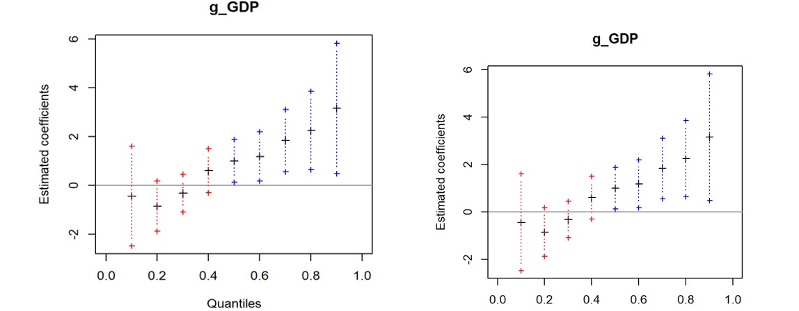
The estimation depicted in Figure 1, Panel A, shows that an increase in RIR (i.e., tighter macrofinancial conditions) is associated with a decrease in the lower quantiles of the GDP growth distribution one period ahead. Hence, the results depicted in Figure 1, Panel A, show the coefficients and their corresponding 95% confidence intervals for a regression of GDP growth on the real interest rate with a 1-period horizon (h=1). Figure 1(b) shows the results from the estimation with a 3-period horizon (h=3). The x-axis displays the GDP growth quantiles corresponding to each coefficient, and the y-axis shows the scale of each coefficient.
Results for the Bahamas
The model was specifically tailored to The Bahamas, and results were computed across various scenarios in which growth fell below the threshold. The expected conditional distribution of growth was estimated for The Bahamas, using the predicted values of the quantile regression (0.05, 0.5, 0.95). The probability of growth falling below the 2.0% threshold was analysed using various scenarios. In this context, various possible macroeconomic shocks and scenarios, depending on the conditions identified as affecting growth prospects, were explored.
An analysis of the baseline, excluding macroeconomic shocks, indicated that the probability of the GDP growth rate falling below the 2.0% threshold is approximately 48.8%. This baseline probability is based solely on the historical distribution of GDP growth rates.
Macroeconomic shock one was assumed to have a 10.0% probability and a size of 5.0%. The results revealed that, in the simulations for a shock size of 0.1, the probability of GDP growth falling below the threshold is consistently high in some scenarios, around 90.7%, indicating a significant impact on economic stability. However, in other scenarios, the probability drops to about 30.0%, highlighting the variability in the effects of this moderate shock size. This suggests that while the economy is highly susceptible to this level of shock in certain conditions, it remains relatively resilient in others.
The second macroeconomic shock was assigned a 20.0% probability and a size of 10.0%. The probability of GDP growth falling below the threshold remains high across several scenarios, similar to the 0.1 shock, reaching 90.7%. However, the probabilities fluctuate slightly more, with some scenarios showing values around 51.5%, indicating a somewhat increased sensitivity to this larger shock size. The outturn suggests that a 10.0% shock generally has a more pronounced impact on economic growth, though the effect still varies across conditions.
In the third macroeconomic shock, a 30.0% probability of a shock was assumed, with a shock size of 15.0%. The probability of GDP growth declining below the threshold remains consistently high in many cases, at 90.7%, but shows higher variability in others, reaching 59.9%. This suggests that the economy faces significant risks under larger shocks, with certain scenarios indicating a considerably higher probability of adverse growth outcomes. The results emphasise the need for robust risk management strategies to mitigate the impact of severe economic shocks.
In summation, the analysis of macroeconomic shocks reveals varying probabilities of adverse GDP growth outcomes. Higher probabilities are associated with larger shock sizes, indicating a more pronounced impact on GDP growth, with the impact decreasing below the 2.0% threshold. Therefore, the results underscore the sensitivity of economic stability to the magnitude and frequency of macroeconomic shocks, highlighting the need for robust risk management strategies to mitigate potential economic downturns.
The study will now examine various macroeconomic scenarios. In macroeconomic scenario one, assuming a scenario probability of 25.0%, a mean growth rate distribution of 2.0%, and a standard deviation of 1.5%, there is approximately a 34.8% chance that GDP growth will fall below the 2.0% threshold. The results indicate that macroeconomic shocks shift the distribution of GDP growth to the left when negative, resulting in larger GDP growth losses.
In macroeconomic scenario two, with a probability of 35.0%, a mean growth rate distribution of 1.5%, and a standard deviation of 2.0%, the probability of GDP growth falling below the 2.0% threshold is around 23.0%. The findings suggest that macroeconomic shocks also shift the distribution of GDP growth to the left, causing GDP growth losses, albeit at a lower rate than in scenario one.
Macroeconomic scenario three features a mean growth rate of 1.0%, a standard deviation of 2.0%, and a scenario probability of 40.0%. Here, the probability of GDP growth declining below the threshold is approximately 9.4%. The results indicate that macroeconomic shocks lead to losses in GDP growth, albeit significantly less severe than in the previous scenarios.
Overall, these scenarios highlight varying probabilities of adverse GDP growth outcomes under distinct macroeconomic conditions. Among the scenarios analysed, those with higher mean growth rates and lower standard deviations are more likely to see GDP growth fall below
the 2.0% threshold. The results across scenarios suggest that macroeconomic conditions significantly influence the severity of potential economic downturns, underscoring the importance of understanding and preparing for variations in economic stability.
Visual Representation of Results
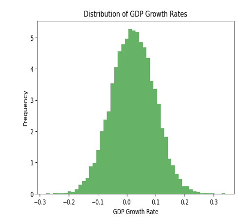
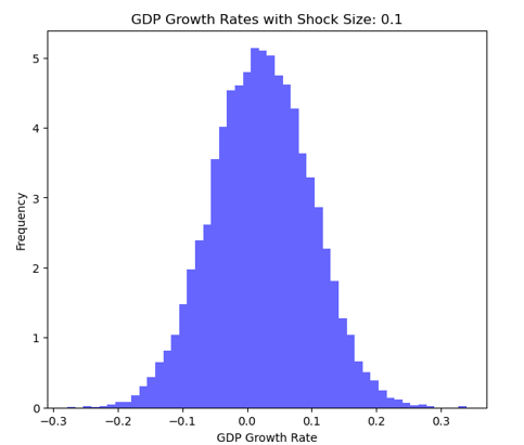
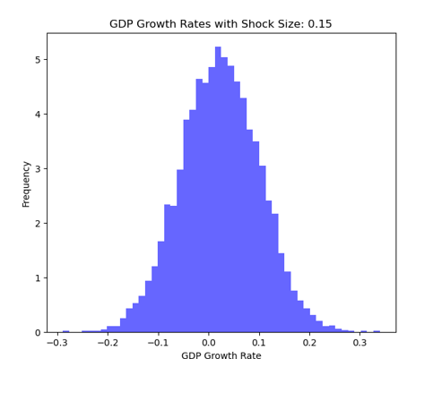
The results from a quantile regression can be visualised and interpreted. Figure 2 shows the distribution of GDP growth rates based on the dataset and visualises the overall behaviour and spread of GDP growth rates without considering any shocks or scenarios for The Bahamas. The x-axis represents the GDP growth rate, which ranges from approximately -0.3 to 0.3. This indicates the rates at which GDP can grow or shrink. Further, the y-axis shows the frequency or count of occurrences of GDP growth rates within each bin. This tells us how often each growth rate occurs in the dataset. Meanwhile, Figure 3 shows the impact of different macroeconomic shock sizes on the probability that GDP growth rates fall below a critical threshold of 0.02.
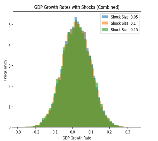
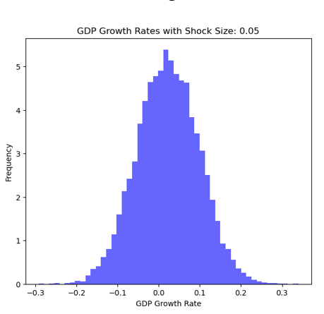
The histograms below, Figures 4-6, show the distribution of GDP growth rates for each shock size (0.05, 0.1, and 0.15). For a shock size of 0.05 (Figure 4), the probability is lower, meaning fewer instances of GDP growth falling below 0.02. As the shock size increases to 0.1 (Figure 5) and 0.15 (Figure
6), the probability increases, showing a higher frequency of adverse GDP growth outcomes. This suggests that larger shocks significantly increase the risk that GDP growth will fall below the threshold.
Policy Implications and Conclusion
Overall, the study revealed that weaker financial conditions are associated with a higher probability of experiencing negative economic growth. In addition, the impact of financial conditions on growth is asymmetric, with a more substantial influence on the lower tail (downside risks) than on the upper tail. The asymmetry suggests a potential trade-off: more relaxed financial conditions may boost short-term growth but heighten vulnerability to future downturns. Country-specific factors, such as financial depth and government effectiveness, can influence the sensitivity of growth to financial risks.
Further, the study showed that, across different levels of macroeconomic shocks, the probability of growth falling below the 2.0% threshold varied by shock size and simulation. Larger shock sizes generally increase the probability that GDP growth will fall below the threshold.
The results are well in line with similar studies conducted. According to Maran [15], early tightening of macroprudential policy would reduce downside (tail) risks to GDP growth by increasing the financial system’s resilience in the medium to long term. The results have several implications for policy-makers, as they dictate how the macro-prudential stance should be adjusted in response to certain macro-financial risks. Various studies support the view that the timing of macroprudential policy is relevant and affects the distribution of GDP growth. Therefore, Galàn [12] recommended tightening the macro-prudential stance when financial conditions become very loose, and the macro- economic environment is strong. Maran [15] also suggested tightening the macro-prudential stance when macro- financial vulnerabilities are sizeable within an expansionary economic environment or when the macro-economic environment improves substantially, as this could lead to the accumulation of macro-financial vulnerabilities in the mid-to-long term, which could negatively impact economic growth [3].
It is evident that the GaR framework can support countries’ macroprudential and macrofinancial policy implementation. The GaR framework has proven it can provide an analytical framework for quantifying the severity of systemic risk based on the current level of macrofinancial vulnerabilities.
Conflict of Interest: The authors declare no conflict of interest. Disclaimer: The views within this paper reflect the thoughts and opinions of the authors and do not represent the views of the Central Bank of The Bahamas.
References
-
Adrian T, Grinberg F, Liang N, Malik S, Yu J (2018) The Term Structure of Growth-at-Risk. IMF Working Paper 14 (3): 283-323.
-
Adrian T, Nina B, Domenico G (2019) Vulnerable Growth. American Economic Review 109(4): 1263-1289.
-
Prasad A, Elekdag SA, Jeasakul P, Lafarguette R, Alter A, et al. (2019) Growth at Risk: Concept and Application in IMF Country Surveillance . IMF Working Paper 2019(36): 39.
-
(2023) Bank of Jamaica. Annual Report_._
-
Busch MO, Sanchez Martinez JM, Rodriguez Martinez A, Montanez Enriquez R, Martinez Jaramillo S (2002) Growth at Risk: Methodology and applications in an open-source platform. Latin American Journal of Central Banking 3(3): 100068.
-
Central Bank of Barbados (2022) Annual Report Bridgetown.
-
Central Bank of The Bahamas Annual Report (2022). Nassau.
-
Chicana D, Nivin R (2022) Evaluating Growth-at-Risk as a tool for monitoring macro-financial risks in the Peruvian economy. Lima: Central Reserve Bank of Peru.
-
Drenkovska M, Volcjak R (2022) Growth-at-Risk and Financial Stability: Concept and Application for Slovenia. Banka Slovenije.
-
European Systemic Risk Board (2019) Features of a macroprudential stance: Initial Considerations.
-
Gachter M, Geiger M, Hasler E (2021) On the Structural Determinants of Growth-at-Risk. Liechtenstein Financial Market Authority.
-
Galan J (2020) The Benefits are at the Tail: Uncovering the impact of Macroprudential policy on Growth-at-risk 74.
-
Lang JH, Izzo C, Fahr S, Ruzicka J (2019) Anticipating the bust: a new cyclical systemic risk indicator to assess the likelihood and severity of financial crises. Occasional Paper Series
-
Lang JH, Marek R, Greiwe M (2023) Medium-term growth-at-risk in the Euro Area. European Central Bank Working Paper Series.
-
Maran R (2023) Impact of macroprudential policy on economic growth in Indonesia: a growth-at-risk approach. Eurasian Economic Review 13: 575-613.
-
(2022) Ministry of Finance Fiscal Policy Paper. Kingston.
-
Obrien M, Wosser M (2021) Growth at Risk and Financial Stability. Financial Stability Notes, Central Bank of Ireland21(2): 1-17.
-
(2021) Regional Central Banks. Regional Financial Stability Report.
-
Schmidt LD, Zhu Y (2016) Quantile Spacings: A simple method for the joint estimation of mulitple quantiles. National Bureau of Economic Research.
-
Škrinjarić T (2024) Growth-at-risk for macroprudential policy stance assessment: a survey. Bank of England Working Paper Series pp: 1-62.
-
Suarez J (2021) Growth-at-risk and macroprudential policy design. Occasional Paper Series pp: 1-37.
-
World Bank (2020) Macro Poverty Outlook, The Bahamas.
-
World Bank (2022) Macro Poverty Outlook Barbados.
-
World Bank (2024) Macro Poverty Outlook Jamaica.
-
World Bank (2024) Macro Poverty Outlook Trinidad and Tobago.
-
Yanchev M (2022) Deep Growth-at-Risk Model: Nowcasting the 2020 Pandemic Lockdown Recession in Small Open Economies. Economic Studies Journal (Ikonomicheski Izsledvania) 31(7): 20-41.
- Community Forestry Enterprises as a Model for Sustainable Forest Development: The Case Of The "Baja Tarahumara" in Chihuahua, Mexico
- Ecological and Socio-Economic Impacts of Chromolaena odorata and Mesosphaerum suaveolens, Two Invasive Alien Species in Central and Southern Benin, West Africa
- Epigenetic Sustainability: Modeling the Human Factor as a Natural Resource through Science 4.0 and the NR3C1 Biological Pilot
- The Rural Territory as a Socioecological System for the Management of Public Policy for Sustainable Rural Development
- Transition Risks in a Small Open Economy: An EDSGE Model with Blue Firms, Financial Frictions and Macroprudential Policy
- Germination Responses of Araribá (Centrolobium tomentosum - Guillem. ex-Bentham - Fabaceae) when Subjected to Different types of Betterments