Computing Spatio - Temporal Water Demand of Wheat Crop Using GIS and Remote Sensing - A Case Study of Faisalabad Irrigation District, Pakistan
Water resources are considered to be finite and their management and judicious use is emerging as a big challenge in the 21st century due to high population growth rate and associated food security. For effective water management of water resources, the assessment of evapotranspiration is necessary. GIS and RS is a best tool to estimate crop evapotranspiration of agricultural crops. The aims and objectives of this study are to compute the real time spatially distributed crop coefficient (Kc) and water demand of wheat crop grown in Faisalabad Irrigation District, Pakistan. In this study monthly crop evapotranspiration for command area was computed using MODIS 13Q1 satellite imagery. The crop evapotranspiration (ETc) was computed by pixel wise multiplication of crop coefficient (Kc) maps and the reference evapotranspiration (ETo) in ERDAS Imagine Model Maker (EIMM). Kc maps were generated from MODIS 13Q1 satellite imagery while reference evapotranspiration (ET0) was estimation using CROPWAT model which compute ETO based FAO-24 modified Blaney-Criddle method using multi variables i.e., temperature, wind speed, sunshine, sun radiations and relative humidity. It was observed that ETc value varied from 0.30-0.89, 0.52-1.47, 0.68-1.64, and 0.61-2.49 mm/day for Dec, Jan, Feb and Mar respectively. Seasonal minimum and maximum value of ETc for wheat crop was 0.30 and 2.49 mm/day for whole command area. It was found that average ETc value for wheat was increased gradually from Dec to Feb as 0.59 to 1.16 mm/days and then decreased to 1.05 mm/days in March. Seasonal crop water requirement of wheat was varied from 265 mm to 665 mm with an average of 465 mm. Results of this study were very close to past studies therefore, it can be concluded that remote sensing based computation of Kc is capable of estimating crop water requirement of the command area satisfactorily for the wheat crop.
Introduction
Irrigation plays an important role in agriculture production, however, with the shortage of water resources agricultural irrigation is not as promising as before and even affects agriculture productivity adversely [1]. Increasing water shortage has led to increase pressure on irrigation engineers to utilize water resources more efficiently for irrigation [2]. To overcome this situation there is an important need to utilize the water resources effectively. Water resources could used effectively with the help of updated data provided by irrigation organization related to crops grown within command area and also the data on quantity of water utilized by crops. But unfortunately access to such type of data is not a simple task because irrigation schemes cover vast area some time thousands of square mile and have large number of farms and data acquisition is more difficult task. GIS and Remote Sensing is a powerful tool for land use and crop identification when used with satellite imagery [3].
Crop evapotranspiration (ETc) represents water demand and governed by weather and crop conditions. Crop evapotranspiration is essential for computation of water balance and irrigation scheduling. Several techniques and models could be used to estimate crop water requirement. CROPWAT model is a better tool to estimate crop water requirement under various climatic scenarios [4]. CROPWAT has widely used in various studies to assess crop water demand and irrigation scheduling of agricultural crops in Greece, Taiwan, Africa, USA, Morocco, Turkey, Zimbabwe and Pakistan [5, 6, 7, 8, 9, 10, 11, 12]. Anadranistakis estimated and validated CROPWAT model for wheat, maize and cotton in Greece [7]. Results of study conducted by Sheng-Feng indicated that crop water requirement predicted by CROPWAT model were effective in management of irrigated water for various crops in Taiwan [8]. Kang reviewed the comparison of various crop water requirement modeling like CROPWAT, MODWht and CERES-Wheat models and concluded that CROPWAT model is better in predicting crop water requirement (CWR) [10]. All of above described models are non-spatial and use point data of (ETo) and Kc from available literatures for computation of crop evapotranspiration [13].
Crop coefficient (Kc) performs an important part in irrigation scheduling and judicial water apportionment. However meteorological data collected from weather stations for estimation of ET are spatially varied highly. Temperature, wind speed, and crop conditions vary up to greater extent within few kilometers in a field and thus effecting crop coefficient and evapotranspiration rate. Therefore, it is essential to make corrections in Kc values as per local conditions. Remote sensing technique resolves this problem because Kc computed from remote sensing reacts to actual crop conditions and captures field to field variability [14]. Advancements in remote surveillance technologies have enabled the acquisition of spatio-temporal hydro-climatic data to estimate actual crop water requirement (ETa) and minimize the uncertainties in predictions [15, 16, 17, 18]. Remote sensing technique provides best estimation of ETc in large irrigation commands area, reliably and economically [19].
ETa computed with satellite data helps to assess the judicial and reliable use of water at big irrigation systems including larger spatial and temporal scales [20, 21, 22]. Tropical Rainfall Measurement Mission (TRMM) based rainfall retrieval supposed to be more reliable than any other remotely sensed estimates [23, 24]. TRMM based rainfall estimations are usually well correlated with the ground based measurements [25, 26, 27]. Moderate Resolution Imaging Spectro radiometer (MODIS) satellite data is helpful to map real time changes in crop coefficient based on indices. Several indices have been used to compute Kc i.e., Normalized difference vegetation indices (NDVI) and soil adjustable vegetation indices (SAVI) [28]. Normalized Difference Vegetation Index (NDVI) has successfully applied in many researches to estimate Kc over large agricultural area to provide real time information about irrigation application [28, 29, 30, 31]. Relationship between crop coefficient and vegetation index must be derived empirically for each type of crop using meteorological data of ET [32, 33, 34]. Both Kc and VI are affected by fractional ground cover leaf area index and must be correlated and Kc could be generated using remote sensing based vegetation indices [35, 36]. Allen explained the development method for estimating crop coefficient. Jayanthi have computed daily evapotranspiration of potato using canopy reflectance based Kc [37, 38]. They used hand-held sensor with high resolution spectral imagery and examined the hydrologic water balance. High resolution aerial imagery of Landsat, MODIS and GOES have used to climax the spatial changes in crop water requirement [39].
In the present study crop water requirement of wheat in District Faisalabad was estimated using NDVI approach. LULC map of study area was obtained from Crop Reporting Service Punjab (CRSP) and wheat class was clipped from map using PCI Geomatica v. 9.3 software and used for further analysis. MODIS13Q1 data was collected from (https://glovis.usgs.gov) and used for computation of Kc of wheat crop. The crop evapotranspiration (ETc) was estimated using the crop coefficient (Kc) and the reference evapotranspiration (ETo) in irrigation command area. Main objectives of this study were (1) To estimate the real time spatially distributed Kc for wheat, and (ii) To estimate spatio- temporal crop water requirement of wheat based on remote sensing derived Kc in command area.
Materials and Methods
Study Area
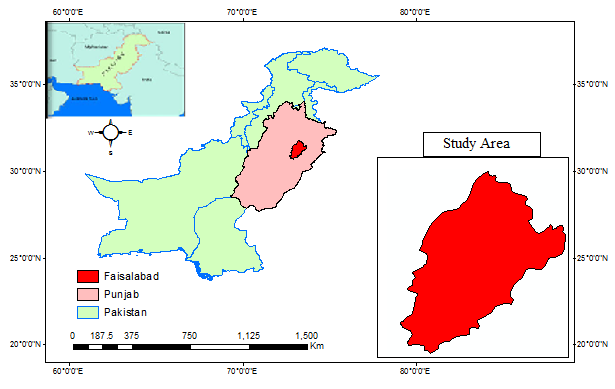
The area under study is District Faisalabad, Pakistan, which is situated between the River Ravi and Chenab which is known as Rechna Doab (Fig. 1). Faisalabad is located at latitude 31° 26’, longitude 71° 06’ and 184.4 m from mean sea level. The total geographic area under study is 5,856 km2. It is designated as subtropical semi- arid region and climate of this area shows seasonal fluctuations in precipitation and temperature. During summer, mean maximum and minimum temperature is recorded as 39 °C and 27 °C respectively. In winter, it reaches up to maximum temperature of 17 °C and minimum 6 °C [40]. The average annual rainfall recorded in the study area is about 300 mm. Major Crops grown in district Faisalabad are wheat, rice, maize and sugarcane. The soils is categorized as medium texture to moderate coarse with favorable permeability and have low organic matter. pH of soil is generally in the range of 8-8.5 and basic in nature. Texture of soil is generally varies in both directions i.e., vertical and horizontal and classified to five series i.e. Nokhar, Jhan, Buchiana, Farida, and Chuharkhana. The topography of study area is relatively considered as flat having about 0.25 m per km in north direction and decreases continuously downward side of Doab. Irrigation system in study area is supply based and discharges of outlets from the distributaries are designed at fixed quantity based on gross command area. Fixed quantity of water is allocated to each farmer based on his land weekly rotational period termed as "Warabandi".
Data Used
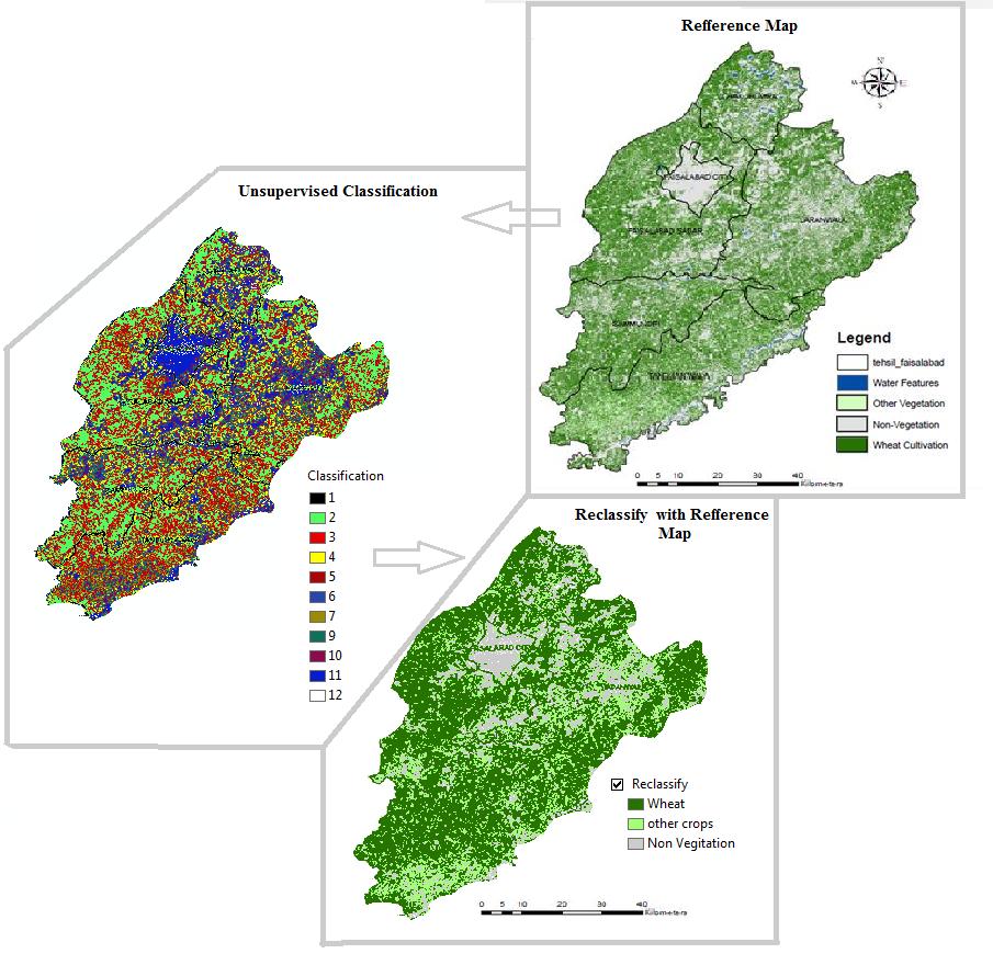
Table 1 illustrated satellite data used in this study to compute the spatially distributed crop coefficient. Time series dataset of 8-day composite MODIS surface reflectance product MOD13Q1 represented by tile numbers 24/5 from December 2015 to March 2016 was acquired from(https://glovis.usgs.gov) for estimation of NDVI index. The data acquired by MODIS13Q1 Aqua &Terra is for every 8days. The imagery MODIS satellites are useful for extracting various information related to vegetation, temperature, clouds, soil moisture, biomass, rocks, minerals and many more. For estimation of reference evapotranspiration (ETo), climatic data of temperature (TMax, TMin and TMean), relative humidity, wind speed, sunshine hours, net radiations and rainfall was obtained from the Metrological observatory of Faisalabad, University of agriculture Faisalabad (Table 2). LULC map of study was collected Crop Reporting Service Punjab (CRSP) (Fig. 2). LULC map of study area contains four land use classes namely; water features, other vegetation, non-vegetation and wheat crop.
| Data type | Month/Year | Date of passing | Resolution | Row/Path | ||||||||||
|---|---|---|---|---|---|---|---|---|---|---|---|---|---|---|
| MODIS 13Q1 | Jan-16 | 25 | 250m | 24/5 | ||||||||||
| MODIS 13Q1 | Feb-16 | 57 | 250m | 24/5 | ||||||||||
| MODIS 13Q1 | Mar-16 | 89 | 250m | 24/5 | ||||||||||
| MODIS 13Q1 | Dec-15 | 361 | 250m | 24/5 |
Table 1: Satellite data used in study.
| Month | T_max | T_min | R.H | WDS | Precp | Sunshine | Net Radiations | ||||||||||||||||
| oC | oC | % | Km/day | mm | hrs | MJ/m²/day | |||||||||||||||||
| Jan | 17.56 | 5.24 | 62.14 | 88.8 | 5.46 | 6.51 | 11.7 | ||||||||||||||||
| Feb | 21.56 | 6.36 | 53.35 | 62.4 | 21.52 | 7.14 | 14.5 | ||||||||||||||||
| Mar | 27.21 | 11.11 | 53.87 | 84 | 44.62 | 8.26 | 18.6 | ||||||||||||||||
| Apr | 34.78 | 19.31 | 33.7 | 122.16 | 13.96 | 10.16 | 23.7 | ||||||||||||||||
| May | 43.23 | 23.98 | 22.17 | 129.6 | 61.23 | 10.23 | 25.1 | ||||||||||||||||
| Jun | 46.11 | 29.34 | 14.82 | 122.4 | 2.17 | 10.7 | 26.1 | ||||||||||||||||
| Jul | 45.45 | 28.76 | 29.11 | 132 | 75.15 | 8.11 | 22 | ||||||||||||||||
| Aug | 43.32 | 26.67 | 35.01 | 115.2 | 31.82 | 9.89 | 23.6 | ||||||||||||||||
| Sep | 39.48 | 20.88 | 27.57 | 112.8 | 5.46 | 8.5 | 19.6 | ||||||||||||||||
| Oct | 34.62 | 15.23 | 26.45 | 74.4 | 0.85 | 8.92 | 17.3 | ||||||||||||||||
| Nov | 27.52 | 11.22 | 38.28 | 69.6 | 0.19 | 8.56 | 14.2 | ||||||||||||||||
| Dec | 21.76 | 7.52 | 49.72 | 55.2 | 0.17 | 4.809 | 9.3 |
Table 2: climate data for the year of 2015-2016 used for computation of ETo.
Data Preprocessing
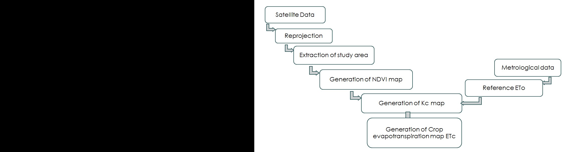
High resolution MODIS satellite images were used to compute Normalized Difference Vegetation Index in study area. For preparation of monthly NDVI maps, total 16 images on 8-days basis were downloaded covering the entire study area. All images were individually projected to WGS1984 system and layer stack to convert them into monthly basis. The images downloaded, cover large areas while the actual area being studied only covers a small portion of the image that’s why required study area was extracted by Mask in GIS software. Stepwise procedure on how to process the data is presented in Figure 3.
Preparation of LULC Map
LULC map of study area was collected from Crop Reporting Service Punjab (CRSP), georefrenced in Arc GIS 10.1. Georefrenced LULC map was classified using unsupervised classification technique. In un-supervised classification technique ISODATA clustering algorithm was applied which classifies the image according to require number of classes and the digital number (DN) of each pixel [41]. After classification, “Reclassify” command in Arc GIS tool box was used to recode the classified areas based on actual map collected from Crop Reporting Service Punjab (CRSP). The study area was classified into wheat class from LULC map in order to use it for further analysis.
Estimation of Normalized Difference Vegetation Index
Vegetation indices (VIs) are mathematical algorithms of different spectral bands, typically in the visible and near-infrared (NIR) which provide composite property of leaf chlorophyll, optical measures of canopy greenness, leaf area, and canopy architecture. Moreover, detection of vegetation pattern and analysis of vegetation health are valuable for monitoring crop vigor and natural resources management [42, 43, 44, 45]. In this study Normalized Difference Vegetation Index (NDVI) was computed from MYD13Q1 imagery. NDVI is a simple numerical index to assess the presence of live green vegetation. NDVI takes the value from -1 to 1. Extreme negative values represent water, values near to zero represent bare soil and values above 0.6 represent dense green vegetation. Firstly digital number (DN) of MYD13Q1 was multiplied with conversion factor in order to estimate NDVI. The following relation was used in order to convert DN into NDVI value.
NDVI = 0.0001 × DN
Where 0.0001 is a conversion factor for MODIS 13Q1 Aqua and Terra. Using vector layers of wheat crop area in GIS software, all four images were clipped (clipping the image for getting area of interest only using PCI Geomatica v. 9.3 software) to get the images representing only wheat crop area. The images representing only wheat cropped area were used to generate normalized difference vegetation index (NDVI).
Estimation of Crop Coefficient (Kc)
Crop coefficient refers to the ratio of well watered crop evapotranspiration and the reference ET, i.e. ETc/ET0, commonly written as “Kc”. Kc value generally can be obtained through field experiments. The Kc values reflect the relative water consumption capacity of crop during different growing stages of different crops. Values of the crop coefficient vary during crop growth stages i.e., its value is generally low during initial growth stage due to less crop cover and reached to maximum when crops fully developed, and remained stable over a period of time and then start to decrease. The method proposed by Brunsell and Gillies to obtain the Kc values for wheat crop was used here [45]. This method computes the Kc based on fraction of vegetation cover and fraction between the emissivity of bare soil and a full canopy.
𝑵𝑫𝑽𝑰−𝑵𝑫𝑽𝑰𝒐
N = 𝑵𝑫𝑽𝑰𝒎𝒂𝒙−𝑵𝑫𝑽𝑰𝒐
Where, NDVI0 = Bare soil NDVI value and NDVI max = Maximum NDVI corresponding to full cover dense vegetation. Then crop coefficient was computed by multiplying “N” two times. Kc = N×N
Estimation of Reference Evapotranspiration (ETo)
Reference ET could be explained as amount of water transpired by well watered short grass with height of 0.12 m, resistance of 70 s/m, and albedo of 0.23. This is very similar to the open surface, highly consistent, vigorously growing, ground cover without the water shortage [37]. Reference evapotranspiration was computed using CROPWAT model which used FAO Penman–Monteith equation to determine the evapotranspiration concerning the hypothetical grass reference surface and provided a standard to which evapotranspiration in different periods of the year.
where ET0 = evaporation rate in units of depth per time; Δ = slope of the saturation vapor pressure versus temperature relationship at Ta; K = short wave radiation net input; L = long wave radiation net input; γ = psychometric constant ≈ 0.066 kPa°C−1; γλv = latent heat of vaporization = 2.45 MJ kg−1; ρw = density of water = 1,000 kgm−3; KE = mass transfer coefficient; va = velocity of air; ea= saturation vapor pressure (at atmospheric temperature); ea = water vapor pressure (in atm). CROPWAT generally required data of multi variables including minimum and maximum temperature, relative humidity, solar radiation, wind speed and the geographic location (altitude and latitude) for the computation of ETO, according to the Penman-Monteith method.
Estimation of Crop Evapotranspiration (ETc)
Crop evapotranspiration is refers to the evapotranspiration of disease free crop grown in large area, not short of fertilizer and water. ETc of wheat crop was estimated by ETO and RS generated Kc values of wheat crop using following equation.
𝐸𝑇𝑐= 𝐾𝑐× 𝐸𝑇0
The steps carried out to estimate the actual crop evapotranspiration from the remotely sensed data are presented through flow diagram in Figure 3.
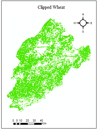
wheat, other crops and non-vegetation. PCI Geomatica v. 9.3 software was used to clip wheat class from LULC map in order to use it for further analysis. Fig. 4 indicated the map of clipped wheat in Faisalabad District. In winter season wheat is the major crop grown in about 702.96 Acres area, which covers about 75% of total cropped area.
Results and Discussion
Land Use Land Cover (LULC) Map Generated for Wheat
The study area was classified into three main classes,
Generation of Normalized Difference Vegetation Index (NDVI) Maps
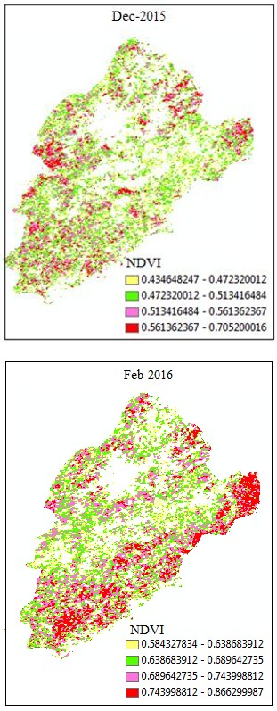
NDVI maps were generated for each month in order to calculate monthly ET of wheat. Seasonal minimum and maximum value of NDVI was 0.4 and 0.9 for whole command area (Fig. 5). Generally, NDVI values for vegetation, water, and bare soil are > 0.1, <0 and 0 to 0.1, respectively. Therefore, most of this study area falls under vegetation condition, as the NDVI value was>0.1. It was observed that NDVI value varies from 0.4-0.7, 0.6-0.9, 0.5- 0.8, and 0.4-0.8 for Dec, Jan, Feb and March. Maximum value of NDVI (0.9) was found in Jan during its development stage. It was found that average NDVI value for wheat was increased gradually from Dec to Jan as 0.56 to 0.77 and then decreased to 0.61 in March. The results obtained were strengthen by comparing with study conducted by Bhadra, Bhadra and Mishra [14, 45]. Results of present study show similarity to past researches conducted on wheat crop. The NDVI value shows spatial changes, which may due to different crop conditions and crop growth stages and sowing dates.
Generation of Crop Coefficient (Kc) Maps
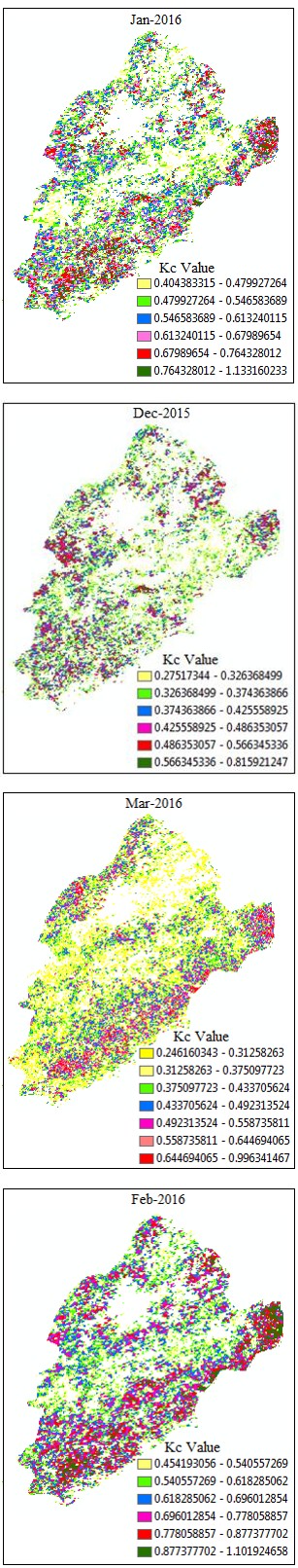
The NDVI maps for different month were generated for irrigation command area and the average values of NDVI were recorded. Kc maps were generated based on fraction of vegetation cover and fraction between the emissivity of bare soil and a full canopy for each month. Seasonal minimum and maximum value of Kc for wheat crop was 0.24 and 1.13 for whole command area (Fig. 6). It was observed that Kc value varies from 0.27-0.81, 0.40- 1.13, 0.45-1.10, and 0.24-0.9 for Dec, Jan, Feb and March. Maximum value of Kc (1.13) was found in Jan during its development stage. It was found that average Kc value for wheat was increased gradually from Dec to Feb as 0.54 to 0.77 and then decreased to 0.60 in March. Similar results has reported by Sirisha, Narendra and Kamlesh and Okran [28, 35, 36]. Sirisha reported that average value Kc of wheat crop varied from 0.29-0.97[28]. The Kc values shows spatial changes, which may due to spatial changes in NDVI which greatly affect as a result of late and early crop sowing.
Generation of Crop Evapotranspiration (ETc)
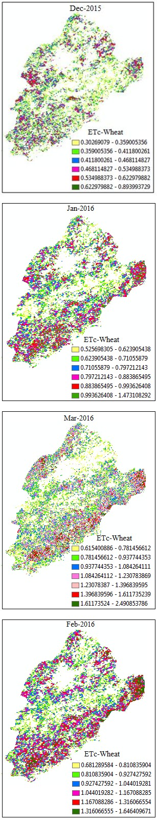
Reference crop evapotranspiration (ETo) values for different months in the phonological period of crop were generated from real-time point meteorological stations. The output of pixel-wise Kc map was multiplied with computed reference evapotranspiration (ETO) for corresponding months to generate the ETc maps (Fig. 7). It was observed that ETc value varied from 0.30-0.89, 0.52-1.47, 0.68-1.64, and 0.61-2.49 mm/day for Dec, Jan, Feb, Mar. Evapotranspiration rate strongly depends on the climate conditions and crop NDVI. Seasonal minimum and maximum value of Kc for wheat crop was 0.30 and 2.49 mm/day for whole command area. Maximum value of ETc (2.49) was found in Jan during its development stage. It was found that average ETc value for wheat was increased gradually from Dec to Feb as 0.59 to 1.16 mm/days and then decreased to 1.05 mm/days in March. ETc shows spatial changes which may due to spatial changes in Kc followed by NDVI.
Seasonal Water Demand of Wheat
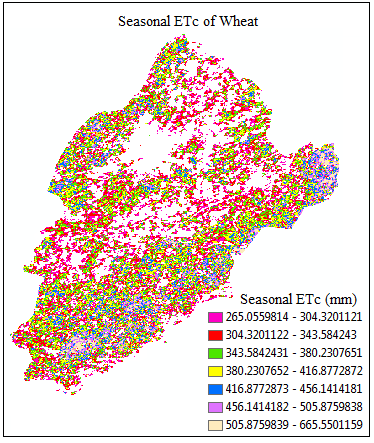
Seasonal total crop irrigation requirement of wheat was computed by pixel wise addition of monthly maps of ETc in ERDAS Imagine 2014, Model Maker. Fig. 8 illustrated spatial changes in crop water demand of wheat crop in Faisalabad Irrigation District, Pakistan. Seasonal crop water requirement of wheat varied from 265 mm to 665 mm.
Seasonal ETc varies spatially which may due to spatial changes in ETo and Kc as a result of NDVI changes and climate conditions. Similar results of estimated ETc were reported by Gontia and Tiwari and Mishra for wheat crop in TSMC command area in West Bengal, India [4, 14]. Therefore, it can be decided that remote sensing based computation of Kc is capable of estimating crop water requirement of the command satisfactorily for the wheat crop.
Conclusions
The present study explores mapping of spatially distributed crop water requirement of wheat crop by using multi-temporal MODIS 13Q1. The pixel wise crop coefficient value was calculated and then combined with metrological estimated reference evapotranspiration. The vegetation indices maps were generated for different months using satellite images. MODIS (Terre and Aqua) satellite can provide data for every 8 days so this methodology can be used for weekly crop evapotranspiration estimation and real time irrigation scheduling. Results of this study revealed that seasonal minimum and maximum value of ETc for wheat crop was 0.30 and 2.49 mm/day for whole command area. It was found that average ETc value for wheat was increased gradually from Dec to Feb as 0.59 to 1.16 mm/days and then decreased to 1.05 mm/days in March. Maximum value of ETc (1.64 mm/day) was found during January- February because during this period wheat crop reaches to developed stage and full canopy cover, results in more consumption of water. Seasonal crop water requirement of wheat was varied from 265 mm to 665 mm with an average of 465 mm. Results of this study were very close to past studies therefore, it can be concluded that remote sensing based computation of Kc is capable of estimating crop water requirement of the command satisfactorily for the wheat crop.
Conflicts of Interest
The authors declare no conflicts of interest.
References
-
Reference ET could be explained as amount of water transpired by well watered short grass with height of 0.12 m, resistance of 70 s/m, and albedo of 0.23. This is very similar to the open surface, highly consistent, vigorously growing, ground cover without the water shortage [37]. Reference evapotranspiration was computed using CROPWAT model which used FAO Penman–Monteith equation to determine the evapotranspiration concerning the hypothetical grass reference surface and provided a standard to which evapotranspiration in different periods of the year. where ET0 = evaporation rate in units of depth per time; Δ = slope of the saturation vapor pressure versus temperature relationship at Ta; K = short wave radiation net input; L = long wave radiation net input; γ = psychometric constant ≈ 0.066 kPa°C−1; γλv = latent heat of vaporization = 2.45 MJ kg−1; ρw = density of water = 1,000 kgm−3; KE = mass transfer coefficient; va = velocity of air; ea= saturation vapor pressure (at atmospheric temperature); ea = water vapor pressure (in atm). CROPWAT generally required data of multi variables including minimum and maximum temperature, relative humidity, solar radiation, wind speed and the geographic location (altitude and latitude) for the computation of ETO, according to the Penman-Monteith method.
- Enhancement of Vegetative Growth and Fruit Yield in Cucumber (Cucumis sativus L.) via Spiritual Blessing (Biofield) Energy Intervention
- Production of Açaí (Euterpe oleracea Mart.) under Different Agroforestry System Management Intensities in Amazonian Floodplain (Varzea) Forests
- Coffee and the Production Region: What is the Secret to the Expression "Quality"?
- Experiential Agripreneurship Training in Sub-Saharan Africa: Integrating a Business Incubator into Postgraduate Livestock Education at the University of Buea
- Advances in Agricultural High-Quality Development
- Linking Compost Residue to ABAGE in Plants - a Short Note