Principal Component Analysis of Hierarchical and Multivariate Data
Principal component analysis concerned with explaining the variance-covariance structure of a set of variables through a few linear combinations of these variables. To determine how many principal components should be considered, the eigenvalues should first be examined. Investigating whether the processing of numbers depend on the way the numbers were presented, i.e. whether the data could be reduced. Four variables (WordDiff, WordSame, ArabicDiff and ArabicSame) were used. Both covariate and correlation matrix were used to obtain the principal components and compare the results between them. In addition, canonical correlation was used to examine the correlation between the set of Word variables and the set of Arabic variables. To see the correlation between the Word variables and Arabic variables, observing the canonical correlation between the first Word canonical variable and the first Arabic variable is enough. Data was reduced into a single principal component (PC1) as more than 80% of the total variability was explained by this principal component.
Introduction
Principal components are independent linear combinations that depend on the correlation or covariance matrix. Principal Component Analysis is concerned with explaining the variance- covariance structure of a set of variables through a few linear combinations of these variables. Its general objectives are data reduction and interpretation [1]. Although p components are required to reproduce the total system variability, often much of this variability can be accounted for by a small number k of the principal components. If so, there is (almost) as much information in the k components as there is in the original p variables. The k principal components can then replace the initial p variables, and the original data set, consisting of n measurements on p variables, is reduced to a data set consisting of n measurements on k principal components [2].
An analysis of principal components often reveals relationships that were not previously suspected and thereby allows interpretations that would not ordinarily result. Analyses of principal components are more of a means to an end rather than an end in themselves, because they frequently serve as intermediate steps in much larger investigations. For example, principal components may be inputs to a multiple regression or cluster analysis, moreover, (scaled) principal components are one “factoring” of the covariance matrix for the factor analysis model considered. To determine how many principal components should be considered, the eigenvalues should first be examined. In this study, both covariate and correlation matrix were used to obtain the principal components and compare the results between them.
Canonical correlation analysis is concerned with the amount of linear relationship between two sets of variables. Sometimes researchers may want to measure two types of variables on each research unit, or may be interested on investigations of the relationship between two sets of variables, like the relationship between the set of academic achievement variables and a set of measure of job success variables, then the canonical correlation analysis is the best method. If we assume that there are Y= (y1, y2. . . yg) and X=(x1, x2, x3, . . . , xg) two sets of variables which were measured on the same sampling unit, the overall correlation between Y and X was obtained using canonical correlation analysis. Canonical correlation is an extension of multiple correlation, which is the correlation between one y and several x’s [3].
Data and Variable Description: Thirty-two subjects were required to make a series of quick numerical judgments about two numbers presented as either two number words (e.g. “two”, “four”) or two single Arabic digits (e.g. “2”, “4”). The subjects were asked to respond “same” if the two numbers had a different parity (one even, one odd). Half of the subjects were assigned a block of Arabic digit trials, followed by a block of number word trials, and half of the subjects received the block of trials in the reverse order. Within each block, the order of “same” and “different” parity trials was randomized for each subject. For each of the four combinations of parity and format, the median reaction times for correct responses were recorded for each subject.
The variables available in the data set are given as:
- WordDiff: is median reaction time for word format and different parity combination.
- WordSame: is median reaction time for word format and same parity combination.
- ArabicDiff: is median reaction time for Arabic format and different parity combination.
- ArabicSame: is median reaction time for Arabic format and same parity combination.
Objectives of the study
As the data were collected to test psychological models of numerical cognition, the main objective of this study was to investigate whether the processing of numbers depend on the way the numbers are presented (word, Arabic digits). In addition, some of specific objectives are: (1). Investigate whether there is possibility to reduce the data. (2). Assess the correlation between the Word variables (WordDiff and WordSame) and Arabic variables (ArabicDiff and ArabicSame). Some important formulas: The correlation between PC (Yj) and the original variables (Xk) were calculated by the formula given bellow.
(1) or Using the standardized formula , = Yj X k e jk j ρ λ (2)
Exploratory Data Analysis: It can be observed from Table 1 that the standard deviation for the variable WordDiff is the highest (190.206) whereas for the variable ArabicSame is the lowest (114.024). The same is true for the mean values of the variables, i.e. 967.562 is the mean value of the median reaction time for word format and different parity combination (WordDiff), which is the highest of all, whereas 710.938 is the mean value of the median reaction time for Arabic format and same parity combination (ArabicSame), and which is the lowest value as compared to the others.
| WordDiff | WordSame | ArabicDiff | ArabicSame | |
|---|---|---|---|---|
| Mean | 967.562 | 875.609 | 825.312 | 710.938 |
| Std | 190.206 | 150.325 | 135.97 | 114.024 |
Table 1: Summary statistics of the variables.
Canonical Correlation Analysis: As results shown in Table 2 (part 2.1), the correlation between the Word and Arabic variables is the largest, being 0.824 between WordSame and ArabicSame. But there are larger within set correlations, i.e. 0.907 between WordDiff and WordSame, and 0.761 between ArabicSame and ArabicDiff.
- Part 2.1 Correlation among the Word and Arabic variables
- Variables
- WordDiff
- WordSame
- ArabicDiff
- ArabicSame
- WordDiff
- 1
- 0.907
- 0.713
- 0.734
- WordSame
- 0.907
- 1
- 0.698
- 0.824
- ArabicDiff
- 0.713
- 0.698
- 1
- 0.761
- ArabicSame
- 0.734
- 0.823
- 0.761
- 1
- Part 2.2 Canonical correlation analysis
- Canonical
- Correlation
- Adjusted Canonical correlation
- Approximate
- Standard Error
- 1
- 0.831
- 0.822
- 0.16
- 0.056
- 0.69
- 2
- 0.333
- 0.111
Table 2: Correlation among the Word and Arabic variables, and canonical correlation analysis.
Picking the largest correlation between Word and Arabic variables is not satisfactory as we lose information in the remaining variables. As a solution to this problem, it is necessary to find a linear combination of Word and Arabic variables, and then discover the correlation between two linear combinations. To avoid possible problems, we find the linear combinations that maximize the correlation.
The first canonical correlation is larger whereas the second one is smaller Table 2 (part 2.2). These canonical correlations are providing us with an overall information for the degree of association between Word and Arabic characteristics. The first correlation 0.831 is slightly larger than the original correlation between Word and Arabic variables, which is 0.824 Table 2 (part 2.2).
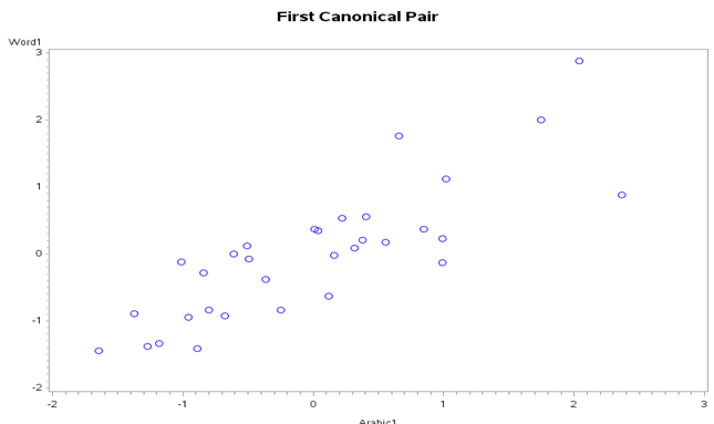
In Figure 1, we can observe that there seems to be a direct linear relation between the first Word canonical variable (WordDiff) and the first Arabic canonical variable (ArabicDiff) indicating correlation. Upon this we can suggest that there may be first canonical correlation between Word variables and Arabic variables.
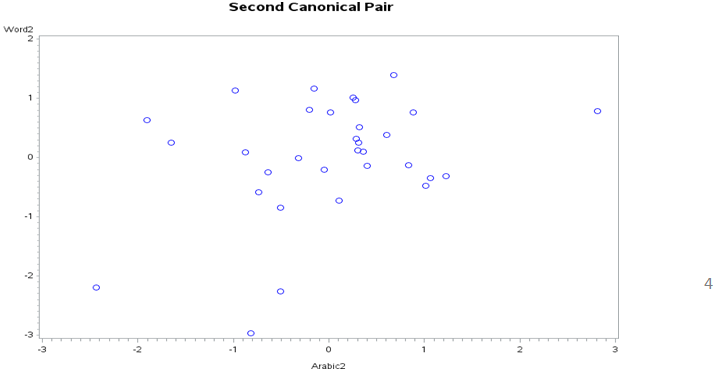
The second canonical pair plot (Figure 2) indicated that there seems no correlation between the second Word canonical variable (WordSame) and the second Arabic canonical variable (ArabicSame). From this, it can be suggested that second canonical correlation is not very important.
It can be done formal tests for canonical correlations. This test assumes normality assumption, and then were obtained by comparing the between (B) and within (W) correlations. The results were presented bellow (Table 3).
| Part 3.1 Eigenvalues of Inv(E)*H=CanRsq/(1-CanRsq | |||||
|---|---|---|---|---|---|
| Eigenvalue | Difference | Proportion | Cumulative | ||
| 1 | 2.2294 | 2.1045 | 0.9469 | 0.9469 | |
| 2 | 0.1249 | 0.0531 | 1 | ||
| Part 3.2 Multivariate Statistics and F Approximations | |||||
| Statistics | Value | F Value | Num df | Den df | Pr>F |
| Wilks’ Lambda | 0.28 | 12.68 | 4 | 56 | <0.0001* |
| Pillai’s Trace | 0.8 | 9.7 | 4 | 58 | <0.0001* |
| Hotelling-Lawley Trace | 2.35 | 16.3 | 4 | 59 | <0.0001* |
| Roy’s Greatest Root | 2.23 | 32.33 | 2 | 29 | <.0001* |
| Part 3.3 Test for canonical correlations in the current row and all that fellow are zero | |||||
| Likelihood | Approximate F | Numerator | Denominator | Pr>F | |
| Ratio | Value | DF | DF | ||
| 1 | 0.275 | 12.68 | 4 | 56 | <0.0001* |
| 2 | 0.889 | 3.62 | 1 | 29 | 0.067 |
Table 3: Formal tests for canonical correlation (CC).
*shows significant at 5% level of significance. Table 3: Formal tests for canonical correlation (CC).
The eigenvalues of Inv(E) were obtained to better investigate the importance of the canonical correlation between Arabic variable and Word variable. As given in Table 3 (Part 3.1), the first canonical pair explains 94.7% of the common structure variability whereas the second canonical pair will probably not be taken into account, because it explains about 5.3% of the variability.
Besides, formal tests were conducted in order to further investigate the importance of canonical correlation. Based on the results of four test statistics shown in Table 3 (part
3.2), as the p-values for all the tests is less than 5% level of significance, we can reject the null hypothesis that canonical correlation equal to zero, and it can be concluded that the canonical correlation between Word variables and Arabic variables is important and then the two sets of variables are linearly related.
Thus, next we identify how many canonical correlation(s) we need, mainly how many canonical correlation(s) are different from zero is done. Based on normality assumption, the null hypothesis is that canonical correlation in the current row and all that follow are zero. Upon the result of likelihood ratio test statistic in Table 3(part 3.3), since p-value <0.0001 for the first canonical correlation is less than 5% significant level, we can reject H0, and conclude that the first canonical correlation is important. For the second canonical correlation coefficient in row 2, since p-value=0,067 is greater than 5% significance level, we do not reject H0 and conclude that the second canonical correlation is not important. Thus, for this study, to explain the correlation between Word variables and Arabic variables, the first canonical correlation is important enough. Since we do not have any information provided on units for the Word and Arabic variables characteristics, it is important to make use of standardized canonical coefficients, which were given in Table 4.
| Part 4.1 | Canonical Coefficients | Correlation | |||||
|---|---|---|---|---|---|---|---|
| Word1 | Word2 | Word1 | Word2 | Arabic1 | Arabic2 | ||
| WordDiff | 0.041 | -2.376 | 0.914 | -0.405 | 0.76 | -0.135 | |
| WordSame | 0.963 | 2.172 | 0.999 | 0.017 | 0.831 | 0.006 | |
| Part 4.2 | Canonical Coefficients | Correlation | |||||
| Arabic1 | Arabic2 | Arabic1 | Arabic2 | Word1 | Word2 | ||
| ArabicDiff | 0.214 | -1.527 | 0.844 | -0.537 | 0.701 | -0.179 | |
| ArabicSame | 0.828 | 1.3 | 0.99 | 0.138 | 0.823 | 0.046 | |
| Part 4.3 | Word canonical variables | Arabic canonical variables | |||||
| Proportion | Cumulative | Proportion | Cumulative | ||||
| 1 | 0.9177 | 0.9177 | 0.6336 | 0.6336 | |||
| 2 | 0.0823 | 1 | 0.0091 | 0.6427 | |||
| Part 4.4 | Arabic canonical variables | Word canonical variables | |||||
| Proportion | Cumulative | Proportion | Cumulative | ||||
| 0.8462 | 0.8462 | 0.5842 | 0.5842 | ||||
| 0.1538 | 1 | 0.0171 | 0.6013 |
Table 4: Standardized canonical coefficients for all the variables and correlations between the original variables and their cano
It is noted in Table 4 (part 4.1) that WordSame variable is important for the first Word canonical variable, providing evidence for correlation between first Word canonical variable and WordSame, since it is observed to be the highest correlation with WordSame, which was found to be important in the first Word canonical variable. Similarly, on Table 4 (part 4.2), it was noticed that in the first Arabic canonical variable, ArabicSame variable is important as it has the highest canonical coefficient in comparison to ArabicDiff. The correlation between first Arabic canonical variable and ArabicSame is also noted to be 0.99. Again looking on the cross correlations between original Arabic variables and the Word canonical variables, we noted that first Word canonical variable has the highest correlation with the ArabicSame, being equal to 0.823, as it was observed to be important in the first Arabic canonical variable.
Moreover, we can notified from Table 4 (part 4.3) that the first canonical pair of Word variables explain 91.8% of the variability in Word variables. Therefore, the canonical redundancy analysis showed that the first Arabic canonical variable is a good overall predictor of the opposite set of variables, the proportions of variance explained being 0.6336. Again in Table 4 (part 4.4) is observed that the first canonical pair of Arabic variable explains a total of 84.6% of the variance in the Arabic variables. The first Word canonical variable is a good overall predictor of the opposite set of variables, the proportions of variance explained being 0.5842. Principal Component Analysis (PCA): Here the principal component analysis is done using both covariance and correlation matrix.
Principal component analysis (PCA) using covariance matrix:
| Part 5.1 | Covariance matrix. | |||
|---|---|---|---|---|
| WordDiff | WordSame | ArabicDiff | ArabicSame | |
| WordDiff | 36178.35081 | 25936.72681 | 18447.56855 | 15909.238 |
| WordSame | 25936.72681 | 22597.75378 | 14261.73085 | 14115.934 |
| ArabicDiff | 18447.56855 | 14261.73085 | 18487.81855 | 11799.73 |
| ArabicSame | 15909.2379 | 14115.93448 | 11799.72984 | 13001.399 |
| Part 5.2 | Eigenvalues and the proportion of variation explained by the PCs | |||
| Eigenvalue | Difference | Proportion | Cumulative | |
| 1 | 76576.3296 | 68696.4479 | 0.8483 | 0.8483 |
| 2 | 7879.8818 | 3650.763 | 0.0873 | 0.9356 |
| 3 | 4229.1188 | 2649.1268 | 0.0469 | 0.9825 |
| 4 | 1579.9921 | 0.0175 | 1 | |
| Part 5.3 | Coefficients of principal components | |||
| PC1 | PC2 | PC3 | PC4 | |
| WordDiff | 0.660421 | -0.46792 | -0.438288 | 0.390894 |
| WordSame | 0.518743 | -0.246012 | 0.414609 | -0.706034 |
| ArabicDiff | 0.409502 | 0.784865 | -0.412483 | -0.214832 |
| ArabicSame | 0.356451 | 0.32329 | 0.68254 | 0.550059 |
| Part 5.4 | Correlations between final principal components and the original variables | |||
| WordDiff | WordSame | ArabicDiff | ArabicSame | |
| PC1 | 0.96082 | 0.95492 | 0.83341 | 0.86507 |
| p-value | <.0001 | <.0001 | <.0001 | <.0001 |
| PC2 | -0.21838 | -0.14527 | 0.5124 | 0.25168 |
| p-value | 0.2299 | 0.4276 | 0.0027 | 0.1647 |
Table 5: Principal component analysis using covariance matrix.
From Table 5 (part 5.1) of the covariance matrix shown that the total variance is 90265.322, and WordDiff and ArabicSame variables have the highest and the lowest variances, respectively. In addition, the total sum of the eigenvalues is 90265.322 which is the sum of the variances of the original variables given in the covariance matrix in part 5.1. It can also be observed from Table 5 (part 5.2) that the first principal component explains about 84.8% of the total variability that is within the rule of thumb, which is at least between 80%-90%. Therefore, the data can be represented by the first principal component with an acceptable loss of information. This first PC can be besides explained by the scree plots and cumulative proportions given in Figure 3.
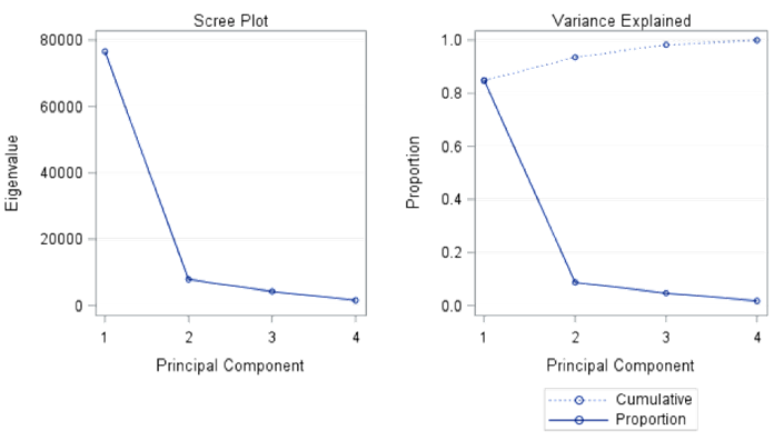
As it can be seen in Figure 3, contribution of the second, third and fourth components are relatively small in comparison to the first principal component. Moreover, the elbow shape occurring at the second PC also proposes only the first PC to be considered. The first PC can be interpreted as the weighted average of all the four original variables. As it can be noticed from Table 5 (part 5.3), WordDiff and WordSame contribute the highest and the lowest respectively as compared to the other variables. The contributions of variables on the first PC can be generalized in the following equation.
- PC1= 0.660WordDiff + 0.518WordSame + 0.409ArabicDiff + 0.356ArabicSame.
- PC2= -0.468WordDiff – 0.246WordSame + 0.785ArabicDiff + 0.323ArabicSame In the second PC, it was shown that the word variables (WordDiff and WordSame) seem to contrast with the Arabic variables. The correlation of the original variables with the respective PCs were given in Table 5 (part 5.4), and the p-value for all of the variables in the first PC is very small (highly significant), which indicated that the original variables are highly correlated with this first PC. The first PC increases as the value for the variables increase and vice versa. On the other hand, in the second PC, it is noticed that as the p-value for the variables WordDiff, Wordsame and ArabicSame is large, the correlation between the original variables and the second PC was found to be insignificant.
Principal Component Analysis Using Covariance Matrix: Instead of making use of the covariance matrix, it is also recommended to use the correlation matrix if the following points are present;
- The original variables are in different scales or units.
- The original variables have high difference in their variability and should be standardized using the correlation matrix.
| Part 6.1 | Correlation matrix | |||
|---|---|---|---|---|
| Variables | WordDiff | WordSame | ArabicDiff | ArabicSame |
| WordDiff | 1 | 0.9071 | 0.7133 | 0.7336 |
| WordSame | 0.9071 | 1 | 0.6977 | 0.8235 |
| ArabicDiff | 0.7133 | 0.6977 | 1 | 0.7611 |
| ArabicSame | 0.7336 | 0.8235 | 0.7611 | 1 |
| Part 6.2 | Eigenvalues and the proportion of variation explained by the PCs | |||
| Eigenvalue | Difference | Proportion | Cumulative | |
| 1 | 3.321 | 2.953 | 0.83 | 0.83 |
| 2 | 0.368 | 0.126 | 0.092 | 0.922 |
| 3 | 0.241 | 0.172 | 0.06 | 0.983 |
| 4 | 0.07 | 0.017 | 1 | |
| Part 6.3 | Coefficients of PCs using correlation matrix | |||
| PC1 | PC2 | PC3 | PC4 | |
| WordDiff | 0.506 | -0.47 | 0.423 | 0.586 |
| WordSame | 0.518 | -0.435 | -0.093 | -0.73 |
| ArabicDiff | 0.475 | 0.731 | 0.463 | -0.158 |
| ArabicSame | 0.499 | 0.233 | -0.773 | 0.314 |
| Part 6.4 | Correlation between the final PCS and the original variables | |||
| PC1 | 0.92273 | 0.94394 | 0.86586 | 0.91045 |
| P-value | <.0001 | <.0001 | <.0001 | <.0001 |
| PC2 | -0.28531 | -0.2642 | 0.4436 | 0.1412 |
| P-value | 0.1135 | 0.144 | 0.011 | 0.4408 |
Table 6: Principal component analysis using correlation matrix.
Sample correlation matrix standardizes the variables and brings them to unit variance as opposed to covariance matrix where the observations with larger units of measurement tend to drive the analysis towards themselves. It is also revealed from Table 1 that the standard deviations are widely spread apart. This suggesting that if a covariance matrix is used, the PCs will be pulled towards such variables with larger standard deviations.
Results in Table 6 (part 6.2) showed that 83% of the total variation is explained by the first PC. Although this result is above the stated rule of thumb value, explaining at least
80% of the total variability, it is lower than the variability explained by the PC using the covariance matrix (Table 5, part 5.2). Furthermore, the first two PCs explain 92.2% of the total variability. Lastly, the first three PCs explain 98.3% of the total variation. As suggested by both the scree plot of Figure 4 and the cumulative proportions represented in Table 6 (part 6.2), the first PC can effectively explain about 83% of the sample variability, leaving only 17% of the sample variability unexplained.
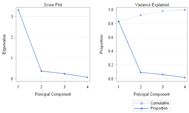
As observed in Figure 4, contribution of the second, third and fourth components are relatively small in comparison to the first PC. In addition, elbow shape occurring in the second PC also suggested only the first PC to be considered. The first PC can summarize the four dimensions in the original data to one dimension with acceptable information loss indicating a data reduction from four dimension to one dimension is reasonable. The PCs can be fitted and interpreted in terms of weighted average of all four original variables as follow.
- PC1= 0.506WordDiff + 0.518WordSame + 0.475ArabicDiff + 0.499ArabicSame
- PC2= -0.470WordDiff – 0.435WordSame + 0.731ArabicDiff + 0.233ArabicSame From PC1, we can observe that the original variables have almost similar contribution for the PC, but in PC2 they have different contribution. Contributions of the original variables to PCs is interpreted by using the correlation between each original variables and the PC. The PC1is strongly correlated with four of the original variables. The PC1 increases with increasing all the four variables. Since the information that can be lost is acceptable, i.e. more than 80% of the total variability is explained by PC1, the data can be reduced into a single PC (PC1).
The scatter plot of the first two PCs under both covariance and correlation coefficient presented in Figures 5 & 6, respectively showed that the two PCs are uncorrelated.
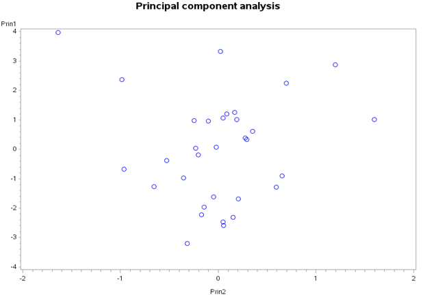
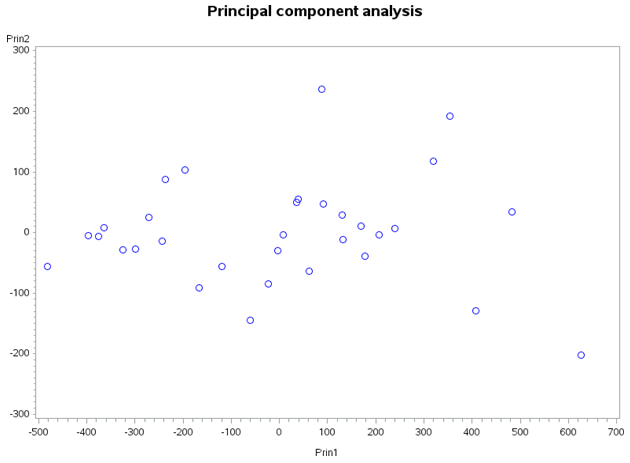
Figure 6: Scatter plot of PC1 against PC2 obtained using correlation matrix. Conclusion Principal components are independent linear combinations that depend on the correlation or covariance matrix. Principal component analysis is concerned with explaining the variance- covariance structure of a set of variables through a few linear combinations of these variables. Canonical correlation analysis is concerned with the amount of linear relationship between two sets of variables. Sometimes researchers may want to measure the correlation between two types of variables on each research unit, or may be interested on investigations of the relationship between two sets of variables, in this case canonical correlation is important. Data were collected from thirty-two subjects on four different variables, i.e. WordDiff, WordSame, ArabicDiff and ArabicSame to make a series of quick numerical judgments about two numbers presented as either two number words (e.g. “two”, “four”) or two single Arabic digits (e.g. “2”, “4”). Objective of this study was to investigate whether there is possibility to reduce the data.
Results indicated that the canonical correlation between Word variables and Arabic variables is high, which is 0.824 between WordSame and ArabicSame. But there are larger within set correlations, which is 0.907 between WordDiff and WordSame and 0.761 between ArabicSame and ArabicDiff. Moreover, we can notified that the first canonical pair of Word variables explain 91.8% of the variability in Word variables. Therefore, the canonical redundancy analysis showed that the first Arabic canonical variable is a good overall predictor of the opposite set of variables, the proportions of variance explained being 0.6336. Again it is observed that the first canonical pair of Arabic variable explains a total of 84.6% of the variance in the Arabic variables. The first Word canonical variable is a good overall predictor of the opposite set of variables, the proportions of variance explained being 0.5842. Moreover, contributions of the original variables to PCs is interpreted by using the correlation between each original variables and the PC. The PC1is strongly correlated with four of the original variables. The PC1 increases with increasing all the four variables. Since the information that can be lost is acceptable, i.e. more than 80% of the total variability is explained by PC1, the data can be reduced into a single PC (PC1).
In conclusion, in order to see the correlation between the Word variables and the Arabic variables, it is adequate to see the canonical correlation between the first Word canonical variable and the first Arabic canonical variable. Data is reduced into a single principal component (PC1) since more than 80% of the total variability is explained by this single PC. Therefore, the information that can be lost will be acceptable.
References
-
Johnson RA, Wichern DW (2000) Applied Multivariate Statistical Analysis. 6th (Edn.), Englewood Cliffs: Prentice- Hall.
-
Jackson JE (1980) Principal Components and Factor Analysis. Component Journal of Quality Technology.
-
Rencher AC (2001) Methods of Multivariate Analysis. 2nd (Edn.), Wiley series in Probability and Statistics.
- Origin, Evolution, and Functional Impact of Short Insertion- Deletion Variants in Human Genomes: A Review
- Harnessing Molecular Glues for Next-Generation Vaccine, Cancer and Cardiovascular Disease Drug Development: A Comprehensive Review
- Lateral Cervical Epidermal Inclusion Cyst in a Paediatric Patient: A Rare Case Report
- Malarial Plasmodium Falciparum with Hepatitis B and C Virus Infections among Blood Donors in Ife Central Local Government Area, Ile Ife, Osun State, Nigeria
- Withanolides and Withaferin A- What’s next in Ashwagandha Research
- Designing of Dual Pulse Photoacoustic Tomography for Imaging of Drug-Response and Tumor Growth