Method for the Estimation of Dilution Efficiency for Water Quality Control, Lake Palic Case Study
In cases of polluted shallow lakes, dilution may provide short term relieve in terms of water quality. However, the efficiency of the dilution technique depends on wide range of influences, making the choice of design parameters quite difficult. The quantifier of mixing coupled with a numerical flow simulator makes a suitable design tool. The combination proved to be sensitive enough to detect even slight differences in the efficiency of dilution between different dilution scenarios. In the presented case study it helped the authors to determine the most suitable location of the emission points for the introduction of clean water into the lake.
Introduction
The number of shallow lowland lakes suffering from eutrophication is increasing [1, 2]. The reasons are, among others, increasing amounts of pollution coming from diffuse and concentrated sources, and changes in temperature and precipitation patterns. In-lake restoration techniques can be applied to ease the pressure. However, not all the available remediation techniques are suitable for shallow lakes. In addition, the right solution is case specific and cost dependent. In general, artificial circulation-increasing aeration, dilution, nutrient diversion, dredging, and nutrient inactivation [1, 3, 4, 5] are some of the appropriate approaches which can provide long-term solutions or short-term relieve in cases of shallow lakes. In this study the possible effects of a short-term solution- dilution of the highly eutrophic Palić Lake by water from the Tisa River – are investigated, exploiting the quantifier of mixing, coupled with a numerical flow model.
The Palić Lake
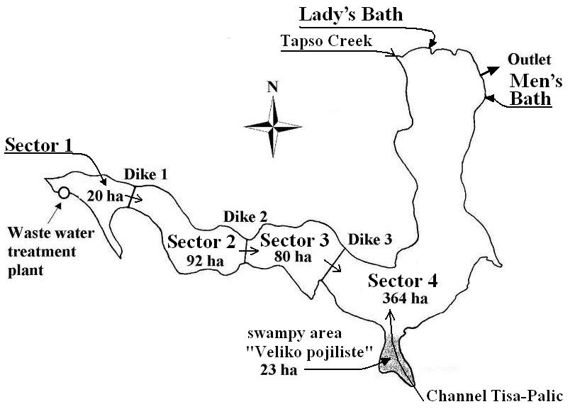
General Description: Palić is a shallow lowland lake in Serbia (between 46o05’52”N, 46o03’39”N and 19o41’39”E, 19o46’01”E). It consists of 4 sectors. The most downstream, Sector 4, is the target of this study. The sectors are connected in series in terms of through- flow, provided by the output of the waste water treatment plant (WWTP) of Subotica. In addition to the input from the WWTP, the Tapso Creek and the Tisa- Palić Channel discharges in Sector 4. A sharp crested weir installed in the Tisa-Palić Channel just upstream to the outlet, decouples the channel from the lake, except for the periods of recharging the lake through the channel by water pumped from the Tisa River.
Such interventions were scarce in the past due to significant losses of water from the unlined channel, setting the cost of the procedure high. The outlet of the lake located in the northeast corner, controlled by a sharp crested weir, maintains water surface elevation within Sector 4 at about 102 MSL (above the Adriatic Sea) (Figure 1).
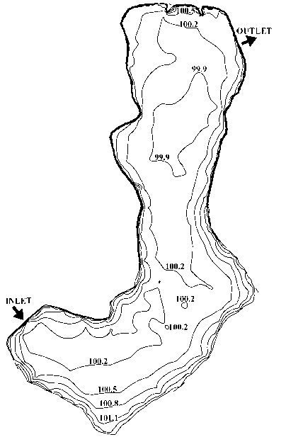
The bathymetry of the actual mud bed was determined by sonar. The corresponding contour map is presented in Figure 2. The basic parameters of Sector 4 are given in Table 1.
| Water surface area at level 102 m MSL above the Adriatic, excluding the shallow swampy area ˝Veliko pojiliste˝ | 365 ha |
|---|---|
| Volume of the lake (V ) at WSL=102 m MSL, mud bed tot | 5843000 m3 |
| Average depth at WSL=102 m MSL, mud bed | 1.60 m |
| Average thickness of the mud | 0.35 m |
| Mean water residence time | ≈200 days |
Table 1: [INLINE_FIGURE:1:1]
The Water Balance of Sector 4
The water balance of Lake Palić corresponding to the arid year 2000 has been analyzed to gain insight into the magnitude of the possible water shortage [6]. Estimated by the stream flow drought of the Sava River in 2000, the return period of this drought was 12.5 r T = years [7]. The water balance equation of the lake regarding Sector 4 is:
$$ Q _ {W W T P} + Q _ {T - P} + Q _ {T C} + (P - E) A - Q _ {O U T} \pm Q _ {G W} = \Delta V \tag {1} $$ where QWWTP is the monthly inflow from the WWTP, QT-P is the monthly inflow from the Tisa-Palić Channel, QTC is the monthly inflow from the Tapso Creek, P is the cumulative monthly precipitation, E is the cumulative monthly evaporation, A is the water surface, QOUT is the monthly outflow through the outlet, QGW is the monthly groundwater inflow/outflow, and ΔV is the monthly change of the lake storage. If ΔV >0 it means gain in storage, while ΔV <0 represents loss of storage during the analyzed month. The analysis has revealed that the highest water deficits show up in June, July and August. In the above table Δz is the change of water surface elevation within the analysed month. In the period from October 1 to March 1, the preferred water level of Sector 4 is 101.7–101.8 m MSL, while it is 101.9–102.1 m MSL for the rest of the year. Based on Table 2, two conclusions come out: a) If the required average summer water level (102.00 m MSL) was provided at the beginning of June, to keep the storage constant (ΔV=_0), interventional discharges of preferably 580500 m3/month, 128193 m3/month, and 1201486 m3/month should have been provided from the Tisa-Palić Channel in June, July and August, respectively. _b) The realized interventional fill of the lake from the Tisa River at a rate of 0 m3/month in June, 747393 m3/month in July and 891886 m3/month in August, none were enough, or were adequately distributed in time.
| S.no | June | July | August | |||||||||
|---|---|---|---|---|---|---|---|---|---|---|---|---|
| 1 | Q (m3/month) WWTP | 0 | 0 | 0 | ||||||||
| 2 | Q (m3/month) T-P | 0 | 747393 | 891886 | ||||||||
| 3 | Q (m3/month) TC | 0 | 0 | 0 | ||||||||
| 4 | P.A (m3/month) | 30960 | 159444 | 33282 | ||||||||
| 5 | E.A (m3/month) | 582822 | 613047 | 575856 | ||||||||
| 6 | Q (m3/month) OUT | 0 | 0 | 0 | ||||||||
| 7 | Q (m3/month) GV | -28638 | 325410 | -658912 | ||||||||
| 8 | WSL, MSL (m) | 101.91–101.76 | 101.76–101.92 | 101.92–101.84 | ||||||||
| 9 | ΔV=AΔz (m3/month) | -580500 | 619200 | -309600 |
Table 2: The elements of the water balance for June, July and August for the arid 2000 Since the quality of water coming from the
In the following, a suitable methodology is presented to quantify the probable efficiency of dilution which could have been achieved by the introduction of clean water from the Tisa River in Sector 4 in the preferred regime, during the June-August period of 2000.
Methodology
numerical modeling is the appropriate tool [8, 9, 10, 11]. It is capable of accounting for a wide range of parameters influencing mixing; in addition, it provides an opportunity for quick analysis of different conditions and design scenarios. In this particular study a numerical model, described in detail [12, 13], and tested on several real-life cases [12, 14] has been used. Since water quality problems are the most severe during droughts, flow conditions corresponding to the arid year 2000 have been simulated. In the case of the Palić Lake, the permanently changing flow patterns promoting water homogenization are dominantly governed by unsteady wind forcing defined by Figures 3, 4 and 5.
For best results, dilution should provide uniform distribution of the clean water introduced within the polluted lake. In the case of the shallow Palić Lake, dilution is mostly dependent on
- the bathymetry influencing flow patterns,
- water balance,
- wind forcing promoting mixing and stirring,
- The location of the emission point at which the clean water is introduced into the lake. The effects of dilution might be estimated posteriorly by measurements. However, for prognostic purposes
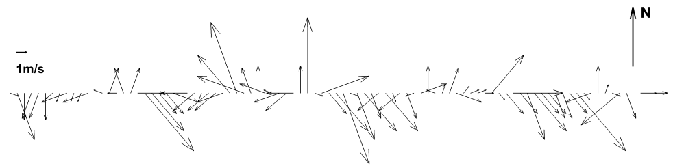
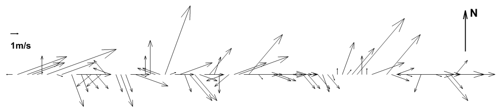
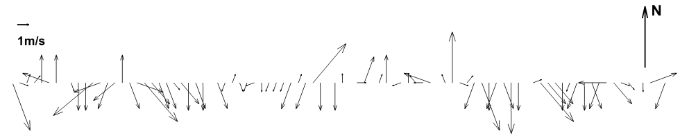
Wind data provided by the Republic Hydro Meteorological Institute of Serbia, and recorded at the meteorological station by the lake has been used.
**Introduction of the River Water and its Distribution in the Lake**
In the case analyzed, the introduction of clean water is by a point source. The location of the emission point (EP) may also affect the efficiency of dilution. Two possible emission points have been investigated in respect to water homogenization: the outlet of the Tisa-Palić Channel and the outlet of the Tapso Creek (see Figure 1). For both emission points the distribution of the river water introduced into the lake was determined by the mentioned numerical model simulating lake currents, generated by the unsteady summer winds (defined by Figures 3, 4 and 5), and the preferred interventional discharges described in the water balance analysis. Water exchange by groundwater flow, precipitation and evaporation was accounted for by the model. However, as the interventional discharges were determined to cover the resultant water losses (to keep the water level constant), no outflow occurred through the outlet during the three months analyzed.
**The Measure of Dilution**
The level of water homogenization at a particular location is quantified by the concentration of the river water within the lake water. If not just a particular location but a larger volume is considered, the average concentration within the control volume might be the appropriate indicator. However, different distribution patterns of clean water within the lake may produce identical average concentrations. Therefore, a certain measure of water homogenization within the volume of interest could give better insight into the efficiency of dilution. In this study the quantifier of mixing (QM) has been exploited to evaluate the efficiency of dilution, introduced and described in detail in Fabian and Budinski [12].
The quantifier of mixing at time $t$, defined as
$$QM = \frac{\frac{V_{occ}^*}{0} - \frac{1}{2} V_{in}^*}{\frac{V_{occ}^*}{0} - \frac{1}{2} V_{in}^*}$$
(2)
Produces values $0 < QM \leq 1$ between states of no mixing (plug flow), and ideal mixing within the volume occupied by the substance of interest. In equation (2), $V$ is volume, $V_{occ}$ is the volume occupied by the substance of interest, $V_{in}$ is the volume introducing the substance of interest, $t$ is time, and $C$ is the volumetric concentration of the substance of interest. Quantities marked with asterisks are normalized; the volume of the lake $V_{tot}$ and the concentration of the substance of interest at the emission point $C_{EP}$, are the reference values chosen for normalization. To reach the value of the QM corresponding to a chosen moment, the map of concentrations of the substance of interest within the lake needs to be produced. Once the map of concentrations is provided, the function of normalized concentration versus normalized volume can be produced, and the QM can be determined by (2). Higher QM values mean higher levels of mixing and vice versa.
To quantify the efficiency of dilution, the quantifier of mixing (QM) was used as described hereafter: the clean water from the Tisa River was taken as the substance of interest. Its concentration was set to 100% at the emission point (EP), where the clean river water is introduced into the lake. By this, the QM evaluates the level of water homogenization at a particular moment. Higher QM values correspond to a rather even distribution of clean water within the lake, indicating more effective dilution, and vice versa for lower QM values.
**Results and Discussion**
The analysis of water homogenization refers to June, July and August of the arid year 2000; however, the flow pattern simulation had begun by May 1st, providing an opportunity for the model to reach a proper flow pattern (initial condition) for the simulation of water homogenization. The initial flow pattern on June 1 is shown in Figure 6.
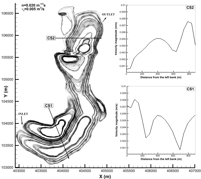
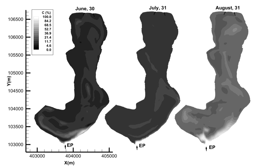
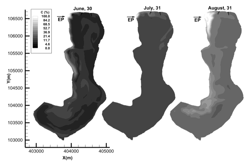
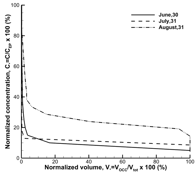
The flow pattern was continuously changing during the simulation period due to unsteady wind forcing, promoting water homogenization. The resulting maps of concentrations for June 30, July 31 and August 31, are shown in Figures 7 & 8, for emission points (denoted by EP on the figures) set at the outlet of the Tisa-Palić Channel and at the outlet of the Tapso Creek, respectively. In Figures 7 and 8 shades of grey are used to represent the actual concentration of river water in the lake water; lighter shades signify a higher concentration of clean river water in a particular spot.
As announced earlier, based on the maps of concentrations, the graphs of normalized concentration versus normalized volume are produced (Figures 9 &
10), and the corresponding values of the QM are calculated (Table 3).

| Emission point (EP) | June, 30 | July, 31 | August, 31 | ||||||||
|---|---|---|---|---|---|---|---|---|---|---|---|
| The outlet of the Tisa-Palić Channel | 0.84 | 0.98 | 0.83 | ||||||||
| The outlet of the Tapso Creek | 0.79 | 0.98 | 0.8 |
Table 3: The comparable values of the QM for the two EPs.
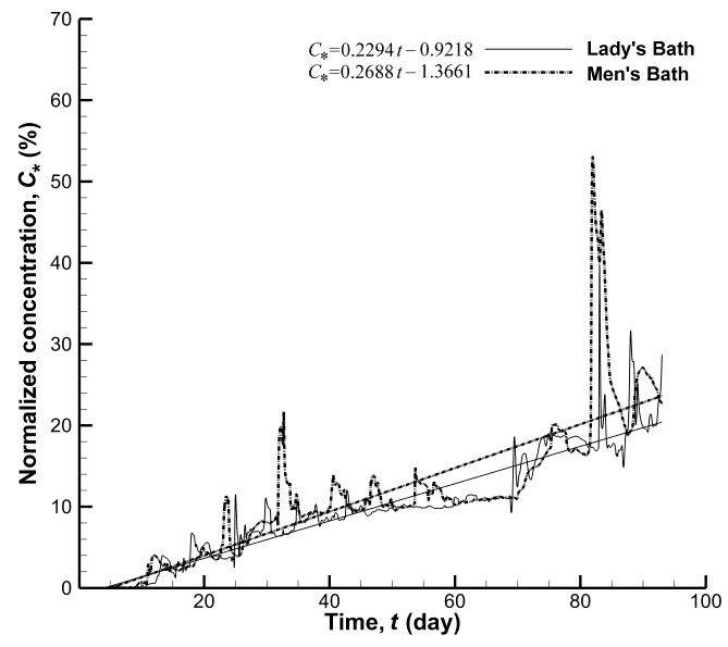
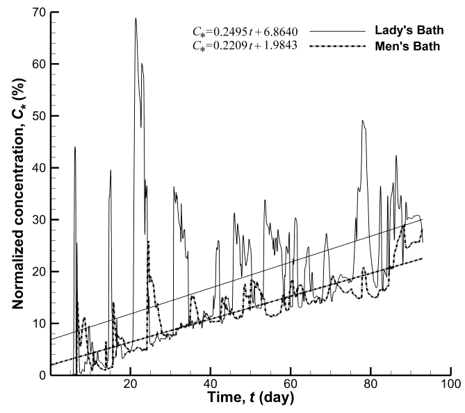
In addition, graphs showing the change of concentration by time, together with the corresponding trend lines and their equations, are provided for two special locations: the Lady's Bath and the Men's Bath (Figures 11 and 12).
The graphs of normalized concentration vs. time (Figures 9 and 10) prove high levels of water homogenization in the cases of both emission points. Clean water spreads successfully all over the lake in less than a month, reaching a concentration of at least 5% at any location of the lake by the end of June. Even though the maps of concentrations (Figures 7 and 8) and the graphs of normalized concentration vs. time (Figures 9 and 10) reflect the effect of dilution, at a glance, no one would tell which EP provides better overall water homogenization. It is especially true to the conditions at the end of July (showing almost no difference between the two EPs), for two reasons:
- The inflow in July was minor (it was just 22% and 11% compared to the inflow in June and August, respectively),
- Meanwhile the July winds were comparable to the winds in June and August, maintaining high levels of water homogenization at all times, resulting in a well homogenized water body at the end of July for both EPs. The values of the QM calculated at the end of July support the above reasoning. Furthermore, they clearly demonstrate that the outlet of the Tisa-Palić Channel makes a better emission point in terms of global water homogenization than the outlet of the Tapso Creek. The differences are not large since the Palić Lake is small and the winds almost continuously generate and
maintain mixing. Wind stillness is present just 7% of the
time.
Regarding the two special locations (the Lady's Bath
and the Men's Bath), both of them closer to the Tapso
Creek EP than to the Tisa-Palić EP, graphs in Figures 11
and 12 provide relevant information. Based on the
equation of the trend lines
$$ C _ {*} = C _ {*} (t) \mathrm {i} $$
in Figures 11 &
12 it can be concluded that mostly the Lady's Bath derives benefit by the vicinity of the Tapso Creek EP. The Men's Bath experiences similar water quality improvement during the analyzed period with both EP locations.
Conclusions
In the presented case study the quantifier of mixing was exploited to determine which location is more suitable for the introduction of clean water into a highly eutrophicated shallow lake in order to maximize water quality improvement by dilution. The quantifier of mixing is a global parameter corresponding to the occupied volume (taken by the substance of interest), sensitive enough to reveal even slight differences by means of quantification. Therefore, it makes an effective tool for solving practical problems concerning water quality.
Acknowledgement
This work was supported by the Ministry of Science and Technological Development, Republic of Serbia (Grant No. 37009), the Municipal Authorities of the City of Subotica, and the Republic Hydro Meteorological Institute of Serbia, who provided wind data.
References
-
Cooke D, Welch B, Peterson A, Nichols A (2005) Restoration and Management of Lakes and Reservoirs. 3rd (Edn.), Taylor & Francis Group, Boca Raton.
-
Lerman A, Imboden DM, Gat JR (1995) Physics and chemistry of lakes. Springer, Heidelberg.
-
Maiss M, Ilmberger J, Zenger A, Münnich KO (1994) ASF6 tracer study of horizontal mixing in Lake Constance. Aquatic Sciences-Research Across Boundaries 56(4):307-328.
-
Peeters F, Wüest A, Piepke G, Imboden DM (1996) Horizontal mixing in lakes. Journal of Geophysical Research/ Oceans 101(C8): 18,361–18,375.
-
Pattantyús ÁM, Tamás T, Tamás K, János J (2008) Mixing properties of a shallow basin due to wind- induced chaotic flow. Advances in Water Resources 31: 525-534.
-
Gabrić O, Kolaković S (2004) Water balance of the Palić Lake. Journal of Faculty of Civil Engineering 13: 44-56.
-
Zelenhasić E (2002) On the Extreme Stream flow Drought Analysis. Water Resources Management 16(2): 105-132.
-
Bahulayan N, Unnikrishnan AS (1992) Simulation of barotropic wind-driven circulation in the upper layers of Bay of Bengal and Andaman Sea during the southwest and northeast monsoon seasons using observed winds. Journal of Earth System Science 101(1): 47-66.
-
Carlos RFJr, David MLMM, Walter C, Carlos EMT, Egbert HvanN (2008) Modelling spatial heterogeneity of phytoplankton in Lake Mangueira, a large shallow subtropical lake in South Brazil. Ecological Modelling. 219: 125-137.
-
Wu J (1980) Wind stress coefficients over the sea surface near neutral conditions-a revisit. Journal of Physical Oceanography 10: 727-740.
-
Weiping H, Sven EJ, Fabing Z (2006) A vertical- compressed three-dimensional ecological model in Lake Taihu, China. Ecological Modelling 190: 367- 398.
-
Fabian J, Budinski Lj (2013) Horizontal Mixing in the Shallow Palic Lake Caused by Steady and Unsteady Winds. Environmental Modeling & Assessment 18(4): 427-438.
-
Budinski Lj, Fabian J (2012) Flow Patterns of Shallow Palic Lake Induced by the Dominant Winds. Architecture and Civil Engineering 10(1): 55-67.
-
Budinski Lj, Spasojević M (2013) 2-D Modeling of Flow and Sediment Interaction - Sediment Mixtures_._ Journal of Waterway, Port, Coastal, Ocean Engineering 140(2): 199-209.
- The Expanding Landscape of Road Rage: A Systematic Review of Conflicts Involving Drivers, Pedestrians, and Micromobility
- Validating Cognitive Models of Royal Navy Performance on Control Systems
- Comparing Standard and State-of-the-art Firefighter Coats on Postural Balance and Gait in a Live Burn Environment
- Investigating the Integration of Telemedicine into Clinicians Workflow: A Review of Methods
- Risk Assessment of Ergonomic Factors in a Textile Firm by RULA, REBA and Fine Kinney Methods
- Impact of Self-Esteem Training on Individuals with Disabilities Aged 17-30