Sensitivity of Stand Density Index to Diameter Calculations and Cutoffs
Stand Density Index (SDI) is a common metric used in forestry to normalize comparisons of disparate size-density relationships and evaluate a stand’s relative density to some maximum. Relative density to some maximum is often used to develop thinning prescriptions for maintaining a forest’s resilience and productivity. However, evaluation of the size-density relationship is fraught with potential for miscommunication given reliance on often differential diameter definitions (size) and common truncation of high density stands (density) with small diameters, depending on the objective of the forest biometrician. The objective of this paper is to highlight commonly used methods for defining a stand’s mean diameter and the multiple approaches to computing stand density index. We explore the traditional definitions of mean diameter and their impact on the computation of SDI: 1) arithmetic, 2) quadratic, 3) Reineke’s diameter by summation, and 4) Reineke’s diameter with Taylor expansion, as a function of differing diameter truncation methods. Our analysis summarizes the strengths and weaknesses of the varying definitional approaches to SDI and emphasizes the need to communicate the objectives for which a particular suite of diameter truncation methods and SDI equations are selected.
Abbreviations
SDI: Stand Density Index; QMD: Quadratic Mean Diameter; AMD: Arithmetic Mean Diameter.
Introduction
Reineke’s stand density index (SDI) was originally developed as the relationship between number of trees per unit area and the average diameter by basal area [1]. This diameter measure used in the original form presented by Reineke is known as the quadratic mean diameter (QMD). That is the classic definition of a quadratic mean [2] where Conceptual Paper QMD is calculated as the “root-mean-square” and expressed as follows:
( ) 2 = = ∑ [1]
n i i d QMD n
1 Where d is the n_th diameter of an individual tree and _n is the total number of trees. When determining QMD from inventory data, it is often necessary to account for expansion factors and should be calculated as follows:
( ) 2 = = ∑ ∑
n * d TPA QMD TPA
i i i n
1 = [2]
i i
1 Where d is the n_th diameter of an individual tree and _TPA is the number of trees per acre represented by that tree. QMD is equivalent to the diameter of the tree of average basal area and can be calculated as follows:
*0.005454 _BA AC QMD TPA = [3]
Where _BA AC is average basal area per acre, TPA is average number of trees per acre and 0.005454 is the constant relating inches to square feet. The quadratic mean diameter is necessarily greater than or equal to the arithmetic mean diameter (AMD), as it gives greater weight to larger trees. The difference between QMD and AMD grows as the stand structure diverges from a tight, unimodal diameter distribution of an even-aged stand, to that of a more skewed or reverse-J shaped distribution of an uneven-aged stand.
For expressing stand attributes, QMD has both mensurational advantages (i.e. the exact relationship to basal area) and historical precedent [3]. Reineke developed SDI from even-aged stands where variance of diameters was low and thus was sufficient for describing ‘average diameter’. The original equation of Reineke SDI was the following:
b QMD SDI TPA = [4]
10 Where TPA is the number of trees per acre, QMD is the classic ‘root-mean-square’ diameter and b is the slope of the self-thinning line. Reineke found this slope, in the linear form of the equation, to be -1.605.
Stage [4] found the disadvantage of SDI in that there was no way to describe the contributions of various diameter classes of trees in the stand to the total index for the stand, and therefore computed SDI as a summation, hereafter referred to as SDI*. The summation method computes SDI* tree by tree within a stand as follows:
b i DBH SDI = ∑ [5]
* 10 Where DBHi is the diameter of the ith tree at breast height in the stand and b is the slope of the self-thinning line, using
1.6 as a good approximation. If SDI* is to be calculated via the summation method from a stand table containing only diameter classes and number of trees, it can be calculated as follows:
i j DBH SDI TPA = ∑
b * * 10 [6]
Where DBHj is the diameter of the jth diameter class in the stand, TPAj is the number of trees per acre in the jth diameter class and b is the slope of the self-thinning line, 1.6 has been a standard approximation. At the plot level, this summation formula is used with each “in” tree’s diameter, and expansion factor as TPA. The plot total is the summation, where the stand total is the average of all plots in the stand.
Zeide [5] describes how the ‘average diameter’ in Reineke’s equation is technically neither the quadratic nor the arithmetic mean, but rather a function of the slope of the self-thinning line, and coined yet another diameter, which he called Reineke’s diameter (DR), calculated as:
1 1 b b R i D d N = ∑
[7]
Where N is the total number of trees, d is the diameters of the i_th tree and _b is the slope of the self- thinning line, with 1.6 as a good approximation. In application, this equation, like that of the summation SDI, needs to be weighted by expansion factors for each tree and should be calculated as follows:
1 1 * b b R i i i D TPA d TPA = ∑ ∑
[8]
Where TPAi is the number of trees per acre represented by the _i_th “in” tree’s diameter. The Reineke diameter can then be used in the classic SDI form in place of QMD, which has been shown to be equal to the summation SDI* [6].
Zeide [5] goes on to present another equation for DR, developed using the first three terms of Taylor expansion, as a function of the arithmetic mean and its variability, represented by the coefficient of variation, as the following:
1 ( ) R b D d C − = +
b b
2 1 1 * 2 [9]
Where d is the arithmetic mean, 𝑏 is the slope of the self-thinning which should lie somewhere between 1, which would produce the arithmetic mean, and 2, which would produce the quadratic mean (1.6 is a good approximation for b), and C2, which is the squared coefficient of variation of the diameter distribution. This form of the DR equation is sometimes written without the coefficient of variation squared [7, 8]. The calculated DR then replaces QMD in Reineke’s SDI equation (Equation [4]) to get at a DR derived SDI.
Shaw [6] demonstrated the significance which stand structure (i.e. shape of the diameter distribution) has on the calculation of SDI. Reineke originally developed the SDI equation from even-aged stand data with normal diameter distributions. The QMD and summation methods produce similar results when applied to even-aged stands but as the diameter distribution becomes more irregular (greater variance about the mean diameter), as found in uneven- aged or multi-cohort stands, these two calculations diverge. Shaw [6] comes to a similar conclusion of that of Zeide [5], that using QMD is not “technically” correct and that the summation method yields the correct result.
Ducey and Larson [9], when attempting to determine if there is a truly “correct stand density index”, concluded that the summation and Reineke’s original SDI should be considered different indices with different properties. Using a two-parameter Weibull function to simulate different diameter distributions with equal number of trees, basal area and QMD, they showed the summation SDI and Reineke SDI are ‘remarkably consistent’ over most of the diameter distributions until the distribution becomes heavily dominated with small trees.
Curtis [10], using real stand data, demonstrated not only how these SDI calculation methods differ with stand structure, but how the diameter cutoff of the input data has a significant impact as well. He concludes that the minimum diameter limit has major effects on calculated density values and that in general trees smaller than 1.6 inches, or all trees of a clearly distinguishable understory, should be excluded from computations.
The overall goal of this analysis is to evaluate the impact of various diameter and SDI equations, as well as diameter cutoffs, on real forest inventory data, and provide context for their impact on assessing relative density of some maximum.
Methods
Data
The forests of western Oregon and Washington will serve as the study area for this analysis. Due to the requirement of the summation SDI and DR equations for individual tree information, rather than plot or stand level summaries, this analysis utilized data from the U.S. Forest Service Inventory and Analysis (FIA) Program from Oregon and Washington, resulting in 10,432 records. FIA subplot data was summarized to the plot level. Tree level information included diameter at breast height (DBH) and number of trees per acre (TPA) represented by each individual tree.
The FIA dataset was summarized to the plot level under three diameter truncations. The first was no diameter cutoff, where all trees with associated expansion factors were included in plot level summaries. The second was the 1.6 inches which Curtis [10] suggested as a reasonable cutoff to reduce issues associated with very large numbers of small trees in the understory. The third cutoff was a larger 5-inch cutoff, although subjective, represents a common small diameter cutoff within forest inventory.
Calculated Metrics
For each plot record, arithmetic mean diameter (AMD), quadratic mean diameter (QMD) and Reineke’s Diameter (DR) via the summation method (Equation [8]), as well as DR via the Taylor expansion (Equation [9]) using both CV and CV2, were calculated. SDI was then calculated utilizing the QMD (Equation [4]) and the three methods for Reineke’s diameter within the classic SDI form (Equations [8] and [9] using both CV and CV2, placed in Equation [4]) as well as SDI* calculated via the summation method (Equation [6]). Ratios of the various calculations were determined for each record under each diameter cutoff.
Results and Discussion
The two diameter cutoffs of 1.6 and 5 inches reduced the number of plots from 10,432 records to 10,423 and 10,285 respectively due to the removal of plots containing only small diameter trees. All mean values of the three calculated diameters increased and number of trees decreased with increasing small tree diameter cutoff (Table 1). The variability in tree diameters, as indicated by the coefficient of variation, decreased with increasing diameter cutoff.
| No Cutoff | >= 1.6 | >= 5 | |
|---|---|---|---|
| DBH (mean) | 8.99 | 9.68 | 12.51 |
| D (summation) R | 10.06 | 10.68 | 13.33 |
| D (CV2) R | 10.18 | 10.79 | 13.39 |
| D (CV) R | 10.52 | 11.23 | 14.14 |
| QMD | 10.77 | 11.36 | 13.89 |
| CV | 0.70 | 0.62 | 0.43 |
| TPA | 404 | 331 | 155 |
| SDI | 282 | 274 | 234 |
| SDI* | 244 | 242 | 219 |
| SDI (CV2) | 252 | 248 | 221 |
| SDI (CV) | 261 | 242 | 252 |
Table 1: Calculated metrics using the various diameter calculations for the different diameter cutoff scenarios.
The increased diameter cutoff causes QMD and AMD to become closer in value. The 50th, 75th and 95th percentiles of the ratio between QMD and AMD get lower as the cutoff increases (Table 2). With a diameter cutoff of 5 inches this ratio stays much closer to 1 with a maximum value of 1.67 compared to the lower and no cutoffs reaching 2.5 and 3 times the difference between QMD and the arithmetic mean.
| Percentile | ||||
|---|---|---|---|---|
| Dataset | 50% | 75% | 95% | Max |
| No Cutoff | 1.2 | 1.36 | 1.7 | 3.02 |
| >=1.6 | 1.16 | 1.29 | 1.56 | 2.52 |
| >=5 | 1.08 | 1.14 | 1.27 | 1.67 |
Table 3: Ratio of QMD to AMD for the different diameter cutoff scenarios.
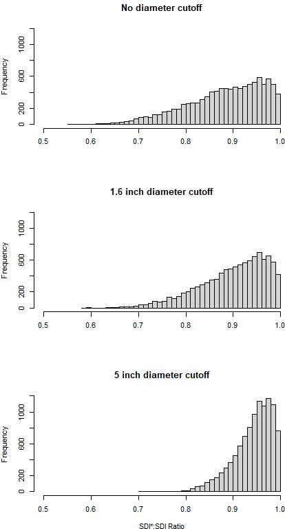
As expected SDI* was always lower than SDI (Table 3), with all diameter cutoffs having a median (50th percentile) ratio between the summation and the QMD (i.e. SDI*:SDI) method of 90% or above. This ratio increased overall as the diameter cutoff increased. This finding is in agreement with Ducey and Larson [9] who concluded the ratio is relatively insensitive to changes to the shape of the diameter distribution until the distribution becomes heavily dominated by small trees. Forest inventories with a minimum merchantability diameter cutoff will decrease sensitivity to small trees with large expansion factors and lead to a ratio of SDI*:SDI close to 1. This ratio may also be utilized to filter for stands of a certain structure. Isaacson [11] used the SDI*:SDI ratio to filter for even-aged, pitch pine stands; where data in their analysis was restricted to any stand with a ratio greater than 0.95.
| Percentile | ||||
|---|---|---|---|---|
| Dataset | Min | 50% | 75% | 95% |
| No Cutoff | 0.55 | 0.9 | 0.95 | 0.98 |
| >=1.6 | 0.57 | 0.91 | 0.96 | 0.99 |
| >=5 | 0.7 | 0.95 | 0.97 | 0.99 |
Ducey [12] demonstrated that the most extreme ratio of SDI* to SDI comes when trees are in two distinct diameter classes, such as those in a two-cohort stand like that of a shelterwood. These are stands where there are large numbers of small trees, yet, with majority of the basal area found in the large diameter classes. The most extreme ratios found in this analysis were between 0.55 and 0.60, with only 0.1% or 11 records falling in this range. For example, the record with the lowest ratio of SDI* to SDI was a plot which contained 14 tree records with six large trees ranging from 30 to 56 inches and eight trees less than 2.5 inches, fitting with the criteria laid out by Ducey [12] and others describing a stand structure which would have an extreme ratio. In this example the QMD derived SDI was 175, and the summation derived SDI* was 96. This same record, with the diameter cutoff of less than 5 inches, SDI and SDI* are almost identical with each at 62. In this extreme example, both the method of calculating SDI and the diameter cutoff are important with regard to any interpretation of what these metrics represent or tell about this stand. Overall, with no diameter cutoff there is a greater amount of records tailing to the lower end whereas the larger diameter cutoff concentrates the distribution closer to 1 (Figure 1).
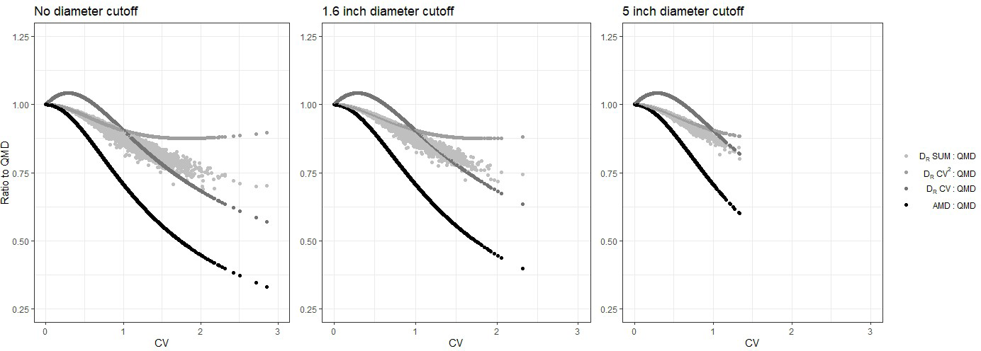
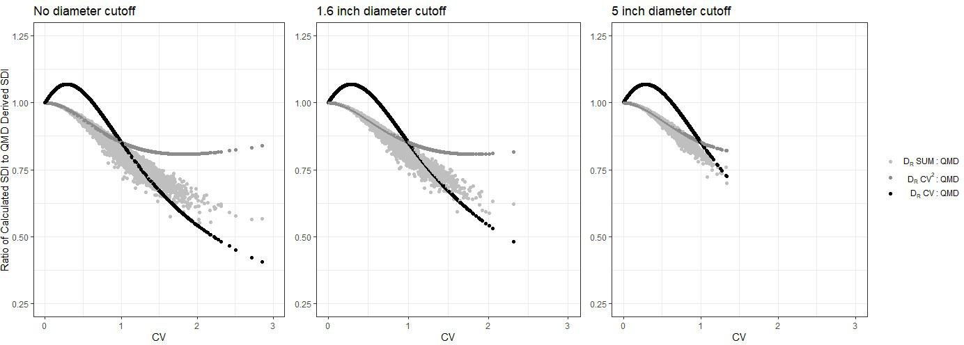
DR calculated from Zeide’s [5] Taylor expansion (Equation [9]) should have the CV squared, proof being that when the b coefficient is 1 DR equals AMD and when b is 2 DR equals the QMD (Figure 2). This proof is only true for QMD when the CV is squared. Although, an investigation into whether DR derived via this method is equal to the summation derived DR, has exposed some issues. First, the assertion and proof shown by Shaw [6], that the summation SDI* (Equation [6]) and the SDI calculated when utilizing the summation derived DR (Equation [8] used in Equation [4]) are equal, is correct. However, DR calculated via the Taylor expansion, as shown in the equations of Zeide [5] where CV is squared or for Weiskittel and Kuehne [7] where CV is not squared, is not exactly equivalent to the DR calculated by the summation method (Figure 3). In particular, as the coefficient of variation about arithmetic mean diameter increases, DR via Taylor expansion increases in proportion to DR calculated via the summation method. Perhaps, the early findings when utilizing DR were developed with stand data having low variability in diameter distribution, where these two calculations are indeed approximately equal. Zeide [5] made use of the stand table in Gingrich [13] (Table 5, p48), which had a coefficient of variation for the smallest and largest diameter classes of 45 and 29 respectively, to calculate DR via Taylor expansion (Equation [9]), which would show close agreement with the summation DR (Equation [8]).
![Figure 2: DR via the Taylor expansion (Equation [9]) when b=2 should be equal to QMD. Coefficient of variation in this equation should be squared. CV on the x-axis is coefficient of variation. Dataset with no diameter cutoff shown.](/fulltextimages/12929/fig_2.png)
Likewise, the SDI found with input of the Taylor expansion DR in place of QMD (Equation[9] using both CV and CV2, placed in Equation [4]) is not equivalent to the SDI* (Equation [6]) found via the summation method (Figure 4). Although, as the diameter cutoff increases there is greater agreement between the summation SDI* and the SDI calculated with DR via the Taylor expansion using CV2, in particular when the coefficient of variation is low. SDI calculated with CV not squared has already been shown to be incorrect, nonetheless it is interesting how the calculated SDI begins to fall in line with the summation SDI* at higher levels of variance. To avoid any confusion about what this diameter calculation is actually representing when calculating SDI*, DR calculated via Taylor expansion should not be utilized. It is recommended to either utilize QMD to calculate SDI, or if an area-based metric is desired, use the summation method to calculate SDI*.
Conclusion
The major conclusion of this analysis is that forest structure and any diameter cutoffs used during forest inventory sampling have a significant impact on SDI or SDI* calculation. Any application of either SDI or SDI* for density management should understand how diameter distributions and truncation could impact the interpretation of these indices, when dealing with irregularly structured forest types [14]. While the use of DR via Taylor expansion has interesting mathematical properties, the findings of this analysis do not support the use of this diameter calculation when applying to the stand density index. If a tree-by-tree, or area-based SDI* is desired, then the summation method, or calculating DR via the summation method, should be utilized. Which diameter calculation to utilize when exploring stand density can have major implications on the modeling process [15]. Ducey and Larson [9] ask whether sensitivity of SDI* to the shape of the diameter distribution enhances the meaning of the index or whether it is meaningless noise. The utility of any density index can only be set by the management objectives it will guide and the meaning it will have on any planned silvicultural activities. Moreover, the structure of the forest will ultimately dictate how the density index will be utilized and interpreted.
References
-
Reineke L (1933) Perfecting a stand-density index for even-aged forests. Journal of Agricultural Research 46(7): 627-638.
-
Iles K, Wilson L (1977) A further neglected mean. Mathematics Teacher 70: 27-28.
-
Curtis R, Marshall D (2000) Why quadratic mean diameter. Western Journal of Applied Forestry 15(3): 137-139.
-
Stage A (1968) A tree-by-tree measure of site utilization for grand fir related to stand density index. USDA Forest Service Research Note INT-77, Intermountain Forest and Range Experiment Station, Ogden, Utah.
-
Zeide B (1983) The mean diameter for stand density index. Canadian Journal of Forest Research 13(5): 1023- 1024.
-
Shaw J (2000) Application of stand density index to irregularly structured stands. Western Journal of Applied Forestry 15(1): 40-42.
-
Weiskittel A, Kuehne C (2019) Evaluating and modeling variation in site-level maximum carrying capacity of mixed-species forests stands in the Acadian Region of northeastern North America. The Forestry Chronicle 95(3): 171-182.
-
Andrews C, Weiskittel A, Amato A, Simons-legaard E (2018) Variation in the maximum stand density index and its linkage to climate in mixed species forests of the North American Acadian Region. Forest Ecology and Management 417: 90-102.
-
Ducey M, Larson B (2003) Is there a correct stand density index? An alternate interpretation. Western Journal of Applied Forestry 18(3): 179-184.
-
Curtis R (2010) Effects of diameter limits and stand structure on relative density indices: a case study. Western Journal of Applied Forestry 25(4): 169-175.
-
Isaacson B, Zipse W, Grabosky J (20240 A density management diagram for pitch pine to illustrate tradeoffs between carbon and wildfire risk. Forest Science 136(1): 53-65.
-
Ducey M (2009) The ratio of additive and traditional stand density indices. Western Journal of Applied Forestry 24(1): 5-10.
-
Gingrich S (1967) Measuring and Evaluating Stocking and Stand Density in Upland Hardwood Forests in the Central States. Forest Science 13(1): 38-53.
-
Chivhenge E, Ray D, Weiskittel A, Woodall C, D’Amato A (2024) Evaluating the development and application of stand density index for the management of complex and adaptive forests. Current Forestry Reports 10: 133-152.
-
Wang Y, Kershaw J, Ducey M, Sun Y, McCarter J (2024) What diameter? What height? Influence of measures of average tree size on area-based allometric volume relationships. Forest Ecosystems 11: 100171.
- Lessons to Learn: Trees are More than the Lungs of the World
- Community Forestry Enterprises as a Model for Sustainable Forest Development: The Case Of The "Baja Tarahumara" in Chihuahua, Mexico
- Ecological and Socio-Economic Impacts of Chromolaena odorata and Mesosphaerum suaveolens, Two Invasive Alien Species in Central and Southern Benin, West Africa
- Epigenetic Sustainability: Modeling the Human Factor as a Natural Resource through Science 4.0 and the NR3C1 Biological Pilot
- Growth-at-Risk: A Framework for Assessing Economic Vulnerability
- The Rural Territory as a Socioecological System for the Management of Public Policy for Sustainable Rural Development