Atmospheric Effects on Spatial Crop Yield Modelling Using Landsat’s Imagery
Remote sensing techniques provide the opportunity for optimizing and predicting crop yields in the field of agriculture. Spatially Yield prediction plays a vital role in Agricultural Policy and provides useful data to policy makers. This paper aims at examining the use of field spectroscopy along with Landsat’s satellite imagery to test the accuracy of raw satellite data and the impact of atmospheric effects on determining crop yield derived from models using remotely sensed data. Vegetation Indices are vital in Crop Yield modelling since they are used in stochastic or empirical models for describing or predicting crop yield. Leaf Area Index, which is also inferred using VI, is also compared to the real values of LAI that are measured using the SunScan instrument, during the satellite’s overpass. The spectroradiometric retrieved Vegetation Indices(VI) of Durum wheat are directly compared to the corresponding VI of Landsat 7 ETM+ and 8 OLI, sourcing from both atmospherically corrected and not corrected satellite images in order to test the effects of atmosphere upon them. Crop Yield is finally determined using the Cyprus Agricultural Research Institute’s Crop Yield model for Durum wheat, adapted to satellite data, and is used to examine the impact of atmospheric effects. The results indicate that if no atmospheric effects algorithms are applied, then there is statistically significant difference in the prediction from the real yield and hence a significant error regarding the model. The study’s goal is to illustrate the need of atmospheric effects removal on remotely sensed data especially for models using satellite images.
Introduction
Field Spectroscopy
Field spectroscopy is a technique used to measure the spectral characteristics of ground surfaces in the natural environment [1]. Field data at or near ground level permit the allocation of points or areas on satellite imagery to corresponding regions on the ground and therefore enables the retrieval of information on the spectral signature of different features [2]. In this study, a field spectroradiometer, GER 1500 was employed, with a range of spectrum from 350 nm to 1050 nm. The general and calibration characteristics of field spectroscopy described by Dekker AG, et al [3]. Spectral signatures can be used to discriminate between healthy and non-healthy vegetation [4, 5, 6, 7, 8].
The role of field spectroscopy has been discussed by Milton and McCoy KR [1, 9]. Field spectroscopy is used to characterize the spectral behavior of ground targets and monitor their suitability as appropriate targets over time. It helps in the inter-calibration of data from different platforms or the calibration of data from the same sensor at different times. Satellite images are used to infer reflectance with and without atmospheric corrections and compare it to the reflectance of a spectroradiometer (which is considered as corrected from atmospheric effects). Ideally, the application of an algorithm for atmospheric compensations, on an image, should finally provide the corrected reflectance which is the reflectance provided from the spectroradiometer.
Crop Yield Modelling
Quantifying crop production at regional scales is critical for a wide range of applications and remote sensing offers great potential for monitoring regional production [10]. Generally, knowledge of crop phenology is combined with multi-temporal imagery to estimate Durum wheat crop yield in the area of interest. Semi- empirical models have been developed to explore crop yield predictions for many different places, including the one used in this paper, which provide valuable information regarding the spatial and temporal distributions of crop production [11, 12]. Figure 1 shows the plots that were used to infer the necessary data.
Crop production is strongly related to many crop, meteorological and environmental factors. Field experiments from the early 1960s have shown that these factors proportionally affect the production of a crop while new experiments have indicated the possibility to estimate a crop’s yield by combining these factors along with remotely sensed data [11, 12, 13, 14]. Therefore, the purpose is to correlate basic factors that affect crop production of Durum Wheat using remote sensing and statistical analysis. The use of remote sensing has been proven to be effective in monitoring the growth of agricultural crops and in irrigation scheduling and efforts have been made to develop various indices for different crops of different regions throughout the globe. The production and prediction of crop yield have a direct impact on year-to-year national and international economies and play an important role in the food management [15].
The semi-empirical model used by Agricultural Research Institute (ARI) for estimating Crop Yield in Cyprus is described in Table 1. It has to be mentioned that the model is best fitted when applied in small scale analysis and when using medium to high resolution satellite imagery (5-30m) where is very effective as mentioned by [16].
| Stage | Model | R2 | SE | F | Sig. | ||||||||||||
|---|---|---|---|---|---|---|---|---|---|---|---|---|---|---|---|---|---|
| Grain filling | y=-0.92+0.37x1- 0.08x2+0.62x3-0.01x4 | 0.886 | 0.12 | 9.085 | 0.002 |
Table 1: Durum wheat Yield Prediction model analysis.
$$ \begin{array}{l} \mathbf {x} 1 = N D V I \\ \mathbf {x} 2 = L A I \\ \end{array} $$
x3= Soil humidity (depth of 40cm)
x4= Crop temperature The model has its best results when applied at the stage of grain filling (stage duration: 8-12 days) with a very high R2 of 0.886 which is a high level of correlation indicating that the independent variables can explain by 88% the dependent variable with standard error of estimate of 0.12 which is very low. The F statistic value is 9.085 indicating that the overall regression model has a good fit for the data since the observed F (9.085) value is higher than the statistic (F4,45=5.7) for p<0.05 illustrating that the hypothesis (Yield can be predicted from NDVI, LAI, Soil Humidity and Crop Temperature) is valid. Significance of 0.002 (less than 0.05) suggest that, overall, the model can statistically significantly predict the outcome variable (Crop Yield). Thus, the prediction model is very accurate and crop yield can be calculated or estimated from the independent parameters NDVI, LAI, SH and CT.
Literature Review
The effects of the atmosphere on spectral signatures and vegetation indices have become an important issue in relevant scientific literature since the 1980s [17]. Atmosphere is a primary source of noise for accurate measurement of surface reflectance with optical remote sensing [18, 19, 20, 21, 22, 23, 24, 25, 26, 27, 28]. Atmospheric effects are a result of molecular scattering and absorption, and influence the quality of the information extracted from remote sensing measurements, such as, vegetation indices. Such errors, caused by atmospheric effects, can increase the uncertainty up to 10%, depending on the spectral channel [29]. Hadjimitsis et al. highlighted the importance of considering atmospheric effects when several vegetation indices, such as NDVI were applied to Landsat TM/ETM+ images for agricultural applications [30]. In their study a mean difference of 18% for the NDVI was recorded before and after the application of darkest pixel method Figure 2.
Therefore, removal of the atmospheric effects is an important pre-processing step required in many remote sensing applications, since it is needed to convert the at- satellite spectral radiances of satellite imagery to them at- surface counterparts [31, 32]. Moreover, if an image is to be used for change detection and monitoring purposes, it is essential that adequate atmospheric and radiometric processing be applied, in order to bring all scenes to a common radiometric datum.
Several atmospheric correction algorithms are found in the literature, ranging from simple to sophisticated [33, 34, 35]. Hadjimitsis et al. classified these algorithms into the following two categories [35]:
- Category (A): Absolute corrections (corrections that lead to surface reflectance). This category can be subdivided into two sub-categories: image-based atmospheric corrections (for example, Darkest Pixel, Covariance Matrix method) and corrections using independent data for atmospheric optical conditions (including in situ measurements or historical records) using physical-based algorithms;
- Category (B): Relative corrections (corrections that do not produce values of surface reflectance).
The problem of atmospheric effects is especially significant when using multi-spectral satellite data for monitoring purposes such as agricultural or land use studies [5, 16]. Hence, it is essential to consider the effect of the atmosphere by applying a reliable and efficient atmospheric correction during pre-processing of digital data. Atmospheric corrections interfere at the stage of pre-processing after Digital Numbers (DN) is converted to Radiance. At this stage atmospheric correction algorithms are applied in order to remove the effects from the atmosphere. A considerable investigation on the effect of the atmosphere on dark targets, in the area of interest, has been already examined; the impact of atmospheric correction on vegetation indices as well on crops as separate targets has been raised and is investigated in this paper [5, 35, 36, 37, 38].
The advantage of the image-based algorithms is the fact that they do not require any ground data during satellite overpass [39]. One of the simplest, fully-imaged based, is the Darkest Pixel (DP) algorithm, categorized in Category (A). The DP principle is based on the assumption that most of the signal reaching a satellite sensor from a dark object, such as, deep inland water bodies (as in the case of the Asprokremmos Dam followed in this study) is contributed to by the atmosphere at visible wavelengths and on the assumption that the near-infrared and middle infrared image data are free of atmospheric scattering effects [39]. Therefore, the pixels from dark targets are indicators of the amount of upwelling path radiance in that band. The atmospheric path radiance adds to the surface radiance of the dark target, giving the target radiance at the sensor. The surface reflectance of the dark target, for the DP algorithm, is approximated to have zero surface reflectance. A modified adaptation of the DP method is to assume a known non-zero surface reflectance of the dark target based on ground truth data (e.g., spectroradiometric measurements).
Objectives
Main objective of the study is to check whereby atmospheric effects can act on yield prediction through remote sensing, a method which is walking over the classic direct methods. Many atmospheric correction methods have been proposed for use with multi-spectral satellite imagery [40]. Such methods consist of image- based methods, methods that use atmospheric modeling and finally those methods that use ground data during the satellite overpass. International literature [2, 7, 41] always premises the need for atmospheric correction on satellite images, especially when it comes to prediction models.
Hence the rhetorical question raised in this study, is “what could happen if atmospheric corrections are not taken into account or if an atmospheric correction algorithm is not working properly”. Never before scientists that apply modelling with the ‘spatial’ parameter have indicated that they use effective atmospheric removal algorithms. The usual path is to apply the model or algorithm onto images of indifferent spatial scales and platforms (for example satellite or UAV image). This paper comes to support modellers and introduce a sound novel methodology for more accurate results. To assist this procedure, authors have used a handheld field spectroradiometer to collect the reflectance of Durum wheat at the time of the satellite overpass in order to compare the correct reflectance (from spectroradiometer) and the reflectance of the satellite images without applying any atmospheric corrections. Based on this the authors have proceeded to estimate vegetation indices, LAI and Crop Yield with and without any atmospheric corrections. Finally, these pairs were compared to find out what could happen to them if atmospheric corrections are not applied to satellite images.
Materials and Methods
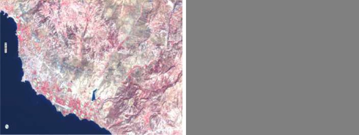
The Study Area
Durum wheat is a vital crop for Cyprus. The main wheat types are the Ourania and Ekavi which are the local types developed by the Agricultural Research Institute of Cyprus. Thus, prediction of wheat production can be useful to policy makers in order to establish policies regarding the market economics. In this study, 25 plots were cultivated with Durum wheat in the district of Paphos province, which were then marked and observed for this study. The area of interest is in the southwest of Cyprus, in a coastal strip between Kouklia and Yeroskipou villages, in the Akhelia area of Pafos. The area is a coastal plain with a seaward slope of about 2% and consists of deep fertile soils. The area is divided by three major rivers, the Ezousa, Xeropotamos and Diarizos. The study area is a traditionally agricultural area with annual and perennial cultivations and is irrigated by Asprokremnos Dam, one of the biggest dams of Cyprus.
The area is almost at sea level (altitude 15 m) and is characterized by mild climate which provides the opportunity for early production of leafy and annual crops. The uniform and moderate temperatures, attributed to the permanent sea breeze of the area, and the relative humidity, are conductive to the early production of fruits and vegetables. Cereals are also cultivated in the area. A typical Mediterranean climate prevails in the area of interest, with hot dry summers from June to September and cool winters from December to March, during which much of the annual rainfall occurs with an average record of 425mm. The whole are is generally homogenous in terms of soil and morphology while the dominant type of soil is the Cambisol (calcic and chromic types).
Wheat in the Akhelia area, Pafos, is sown in late November to mid-December using a sowing machine. In general, the study area is rainfed but, under severe drought conditions, is irrigated. The fields are treated with a basic 20:20:0 fertilizer upon sowing and again at a later time receive an additional top fertilization using a 34.5:0:0 formula. After the 4th leaf, the study area is treated with a wheat-triticale specific pesticide that controls both broad and narrow leaf weeds. The model application is taking place at the grain filling stage which is normally in the beginning of April and ends in the mid- April.
Overall Methodology
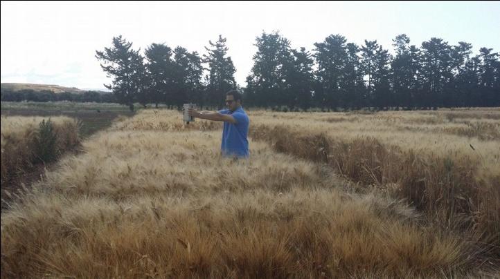
The overall methodology lies in two levels: a) estimating Vegetation Indices along with LAI and Crop Yield using satellite images, field spectroscopy techniques and the Crop Yield prediction model and other instruments and b) comparing using statistical techniques these factors (VI, LAI and Crop Yield) to the real values for inferring the effects of atmosphere on the procedure for predicting Crop Yield using remotely sensed data . More analytically, the methodology can be categorized in the following four steps (a) to (d): a) A field campaign, using a field spectroradiometer, was undertaken in the area of interest (25 plots cultivated with Durum wheat) during April 2013 and 2014 to coincide with the periods of grain filling where is the period where the ARI’s model is applied. In this research, the method of using a white reference panel described by McCoy KR and was adopted Milton EJ [9, 42]. The GER1500 was used to acquire measurements on the target and on the control panel. By applying the ratio of the reflected radiance from the target to the reflected radiance from the panel and by taking into account the control panel correction, the reflectance of the target was obtained. Field spectroradiometric measurements were collected in-situ using the GER-1500 field spectroradiometer with reflectance spectrum ranging from 350 nm to 1050 nm. The instrument’s field of view was 4o so the user was taking measurements of 1,2 m above the target (8 cm).
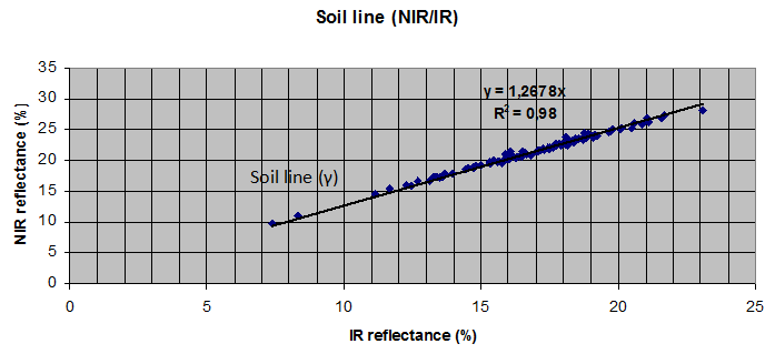
Using the GER1500 spectro-radiometer in situ, the surface reflectance values equivalent to the Landsat 8 OLI or/and ETM+ RED and NIR bands were determined. To filter the data through the Relative Spectral Response (RSR) values of Landsat 8 OLI/ETM+, the GER1500 reflectance values were interpolated to obtain the reflectance values at the incremental wavelength of the RSR. This was done since the GER1500 reflectance values were given at a different incremental wavelength scale. Then, the GER 1500 experimental data was filtered through the RSR functions and averaged within the limits of the RED and NIR 8 OLI/ETM+ bands, to yield the in- band reflectance values. Vegetation indices were determined for each date of acquisition and averaged to have the average value of the grain filling stage At each time, about 25 in situ measurements well spread in each plot, were collected in order to have a representative sample from the plot. Then the 25 measurements were averaged into a single representative measurement which was then processed to retrieve NDVI and WDVI. Simultaneously to spectroradiometric measurements, LAI measurements were taken using the SUN-SCAN canopy analyzer (Delta-T Devices Ltd., UK). The same procedure for averaging the LAI data has been followed and averaged LAI values have been created for each of the plots for the grain filling stage for each year. b) The field data was collected on schedule based on the satellite overpass in order to have comparable to the satellite imagery data. The satellite overpass was at the specific dates for 2013 (5, 13 and 21 of April for ETM+, 8 OLI and ETM+ respectively) and for 2014 (1 and 16 of April for 8 OLI and 8 OLI respectively). Thus averaged spectroradiometric data and averaged Landsat’s remotely sensed data regarding NDVI and WDVI of the grain filling stage of the Durum wheat have been prepared for each of the 25 plots in the area of interest. The WDVI index has the advantage to reduce to a great extent the influence of soil background on the surface reflectance values. Although simple, WDVI is as efficient as most of the slope based VI. The effect of weighting the red band with the slope of the soil line is the maximization of the vegetation signal in the near-infrared band and the minimization of the effect of soil brightness. After creating a set of data from bare soil of the area during the year, the slope of the line was set to 1.27. The slope line is created from the NIR and R spectrum using spectroradiometric data (200 sample random measurements) from the area’s soil (Figure 4).
ERDAS imagine (version 11) was used for the pre-processing and post-processing of satellite images. All satellite images were geo-referenced using a second order polynomial with 12 ground control points. Then all images have undergone atmospheric correction using the Darkest Pixel algorithm. The algorithm of Darkest pixel has been applied to each satellite images as for atmospheric effects removal. After the Digital Numbers (DN) of the selected dark target (Asprokremmos dam in the area of interest) near the area of interest are converted to units of radiance using calibration offset and gain parameters, the target reflectance at ground level is determined using the following simplified equation:
- Where
- $\rho g$ is the target reflectance at the ground
- Lds is the dark object radiance at the sensor
- Lts is the target radiance at the sensor,
- Eo.d is the solar irradiance at the top of the atmosphere corrected for earth-sun distance variation
- $\theta$ is the solar zenith angle
It is important to mention that dark object radiance at the sensor corresponds to the atmospheric path radiance which is subtracted or added from each spectral band from the target radiance at the sensor.
Also, LAI of the specific plots was estimated to be compared to the real values LAI which were measured from field measurements. For estimating LAI the following equation was applied [4; 43]:
$$LAI = -\frac{1}{a} \ln \left( 1 - \frac{WDVI}{\rho \infty (\lambda nir)} \right)$$
- Where
- LAI = Leaf Area Index,
- WDVI = Weighted Difference Vegetation Index,
- $\alpha$ = complex combination of extinction and scattering coefficients,
- $\rho \infty$ = asymptotically limiting value of the WDVI at very high LAI values.
Standard Values for $\alpha$ and $\rho \infty$ were taken from literature specifically for cereals, and used for the model [44;45].
The specific equation was applied to satellite images and LAI maps were created. Various studies have shown that empirical equations of LAI and Vegetation Indices can provide good estimates of LAI from the satellite images [4, 37, 43, 44, 45, 46].
c) Then the Crop Yield Prediction model has been applied by using atmospheric corrected and non-corrected available satellite imagery of April 3013 and 2014 mentioned earlier. In the model application LAI and NDVI are estimated using the satellite images while the other two factors, namely soil humidity and crop temperature were directly measured and averaged in each plot. Leaf Area Index (LAI), crop temperature and soil humidity at 40cm in situ measurements were also taken simultaneously to spectroradiometric measurements. Using the SUN-SCAN canopy analyzer (Delta-T Devices Ltd., UK), users can acquire the LAI value directly by setting it up perpendicular to the crop rows [47]. As well, a calibration measurement above the canopy is needed for each time the user takes a measurement in the crops. The SunScan was calibrated under a standard light source against an accurate Photosynthetic Active Radiation (PAR) quantum sensor. The spectral and cosine responses of the sensors approximate to the ideal response, but fall off at the extremes of the range. Under most normal daylight conditions, errors due to the deviation are small, but it is possible, in conditions such as under artificial light, to find larger errors in the absolute values measured. Since the Sunshine Sensor and Probe are closely matched, this has minimal effect on the canopy calculations which are based on ratios of incident and transmitted light [48]. Crop temperature (CT) was derived from a digital handheld thermometer while soil humidity (SH) was derived from soil moisture WET-2 from Delta Devices. Then, values of real Crop Yield along with estimated Crop Yield from corrected and not corrected satellite images have been created for every single plot for each year (2013 and 2014). These values, again, are the average values for the specific period of grain filling. The final product of the model application is a Crop Yield map for each satellite image, where values of Durum wheat yield are retrieved and recorded in the tables next to the real yield values, given from the Agricultural Research Institute of Cyprus.
d) Finally for each factor affecting Crop Yield but also for Crop Yield, a statistical method for comparing the paired values have been employed, in order to test if there is significant differences among the different pairs. Student’s t-test is used to find out basically if there is statistically significant difference between real and corrected values, real and uncorrected values and lastly between corrected and uncorrected values. The Student’s t-test for paired samples, as a statistical significance test, was applied to compare and assess the results meaning. To assess the value of t, the standard deviation SD of each pair of values (real and predicted) must be known. Dj refers to the difference of each pair, Da is the average difference of each pair and n is the number of the pairs.
2 D S Variance ( ) is calculated from equation (1):
(𝜮𝑫𝒋)𝟐
𝟐−
𝟐= 𝜮𝑫𝒋
𝒏 / 𝒏−𝟏) (1) 𝒔𝑫
2 Da S Following, the average Variance ( ) of all pairs must be calculated from the following equation (2)
𝟐 = 𝒔𝑫
𝟐/𝒏 (2) Finally, t value is calculated solving equation 3:
𝒔𝑫𝒂 𝑫𝒂
𝒕= 𝑺𝑫𝒂 (3)
Results and Discussion
Spectroradiometric measurements were processed in order to derive the ‘at satellite reflectance’ which is a comparable form of reflectance to the reflectance of Landsat 7 ETM+ and 8 OLI satellites respectively, which are the satellite images used for this study. The specific spectrum was used to infer the necessary data to create the two VI (NDVI, WDVI for estimating LAI) which are needed as inputs to the model predicting the Durum wheat’s yield. This paper examines the impact of atmospheric effects on the specific model. Though, one more step is taken from the authors in order to realize how the intervening atmosphere affects the Vegetation Indices and LAI which in turn affect the model application. The results have indicated that atmospheric effects must always be removed from the satellite imagery otherwise the results can be seriously misleading. For all the cases, successful atmospheric removals have led to values which have no statistically significant difference from the real values of the factors taken under study in this paper while satellite images that have not undergone any atmospheric removal have always huge differences from the real or compensated (corrected) values.
Using the Student’s T-test, a comparison for VIs, LAI and Crop Yield has been conducted between the real and corrected values, between the real and uncorrected values and finally between the corrected and the uncorrected values for all the cases. There were no comparisons for the other two factors of Crop Yield model, crop temperature and soil humidity, since they were directly measured and averaged in the field and not estimated from the remotely sensed data. As mentioned before, T-test has revealed that if raw satellite data is used without any effective atmospheric removals, then the results are very misleading with significant differences from the real values.
Table 2 and 3 illustrate the values of each factor for the real, the corrected and the raw (uncorrected) values which have been used to test what is the effect of atmosphere on the procedure for estimating Crop Yield of Durum wheat using satellite images. Table 2 refers to year 2013 and Table 3 to 2014. For each factor (NDVI, WDVI, LAI and Crop Yield) there are 3 columns recorded. The radiometric (or real), the corrected and the uncorrected values. The radiometric value is the real value of the factor and it will be the reference value for the other two.
| NDVI | NDVI | NDVI | WDVI | WDVI | WDVI | CROP YIELD | CROP YIELD | CROP YIELD | LAI | LAI | LAI | |
|---|---|---|---|---|---|---|---|---|---|---|---|---|
| PLOTS | RADIOMETRIC | UNCORRECTED | CORRECTED | RADIOMETRIC | UNCORRECTED | CORRECTED | CORRECTED | UNCORRECTED | REAL | CORRECTED | UNCORRECTED | REAL |
| 1 | 0.67 | 0.61 | 0.66 | 0.53 | 0.44 | 0.55 | 1.71 | 1.83 | 1.67 | 4.01 | 2.75 | 4.10 |
| 2 | 0.69 | 0.60 | 0.67 | 0.54 | 0.45 | 0.56 | 1.72 | 1.82 | 1.68 | 4.01 | 2.85 | 4.20 |
| 3 | 0.74 | 0.59 | 0.74 | 0.59 | 0.46 | 0.60 | 1.70 | 1.82 | 1.67 | 4.45 | 2.95 | 4.30 |
| 4 | 0.70 | 0.62 | 0.72 | 0.54 | 0.45 | 0.55 | 1.71 | 1.83 | 1.69 | 3.50 | 2.85 | 3.60 |
| 5 | 0.75 | 0.65 | 0.77 | 0.61 | 0.45 | 0.60 | 1.70 | 1.83 | 1.69 | 4.61 | 2.85 | 4.40 |
| 6 | 0.78 | 0.64 | 0.79 | 0.62 | 0.46 | 0.61 | 1.70 | 1.82 | 1.69 | 4.96 | 2.95 | 4.60 |
| 7 | 0.61 | 0.60 | 0.60 | 0.51 | 0.47 | 0.53 | 1.73 | 1.81 | 1.72 | 3.16 | 3.05 | 3.00 |
| 8 | 0.64 | 0.69 | 0.63 | 0.52 | 0.47 | 0.54 | 1.73 | 1.82 | 1.73 | 3.16 | 3.05 | 3.00 |
| 9 | 0.78 | 0.69 | 0.76 | 0.62 | 0.49 | 0.60 | 1.68 | 1.83 | 1.70 | 4.78 | 3.27 | 3.90 |
| 10 | 0.63 | 0.71 | 0.64 | 0.52 | 0.48 | 0.50 | 1.70 | 1.84 | 1.73 | 3.38 | 3.16 | 3.50 |
| 11 | 0.65 | 0.54 | 0.64 | 0.53 | 0.48 | 0.52 | 1.71 | 1.75 | 1.74 | 3.38 | 3.16 | 3.50 |
| 12 | 0.66 | 0.55 | 0.64 | 0.53 | 0.51 | 0.52 | 1.71 | 1.76 | 1.74 | 3.50 | 3.50 | 3.60 |
| 13 | 0.66 | 0.54 | 0.64 | 0.54 | 0.50 | 0.54 | 1.72 | 1.77 | 1.75 | 3.88 | 3.38 | 3.60 |
| 14 | 0.71 | 0.56 | 0.70 | 0.54 | 0.49 | 0.54 | 1.73 | 1.78 | 1.76 | 3.88 | 3.27 | 3.70 |
| 15 | 0.72 | 0.55 | 0.71 | 0.54 | 0.49 | 0.55 | 1.69 | 1.75 | 1.73 | 3.62 | 3.27 | 3.50 |
| 16 | 0.66 | 0.55 | 0.64 | 0.53 | 0.51 | 0.52 | 1.73 | 1.77 | 1.77 | 3.62 | 3.50 | 3.60 |
| 17 | 0.61 | 0.50 | 0.60 | 0.51 | 0.49 | 0.48 | 1.74 | 1.72 | 1.79 | 3.16 | 3.27 | 3.30 |
| 18 | 0.60 | 0.51 | 0.60 | 0.50 | 0.53 | 0.47 | 1.71 | 1.71 | 1.74 | 3.16 | 3.75 | 3.30 |
| 19 | 0.58 | 0.52 | 0.59 | 0.49 | 0.54 | 0.46 | 1.71 | 1.73 | 1.75 | 2.95 | 3.88 | 3.20 |
| 20 | 0.60 | 0.50 | 0.60 | 0.50 | 0.52 | 0.47 | 1.75 | 1.69 | 1.78 | 2.95 | 3.62 | 3.30 |
| 21 | 0.62 | 0.55 | 0.61 | 0.51 | 0.55 | 0.49 | 1.76 | 1.78 | 1.79 | 2.85 | 4.01 | 3.20 |
| 22 | 0.68 | 0.56 | 0.69 | 0.54 | 0.48 | 0.53 | 1.75 | 1.79 | 1.79 | 3.16 | 3.16 | 3.20 |
| 23 | 0.71 | 0.54 | 0.70 | 0.54 | 0.47 | 0.52 | 1.82 | 1.81 | 1.84 | 3.27 | 3.05 | 3.20 |
| 24 | 0.73 | 0.55 | 0.73 | 0.56 | 0.44 | 0.56 | 1.82 | 1.81 | 1.83 | 3.50 | 2.75 | 3.30 |
| 25 | 0.76 | 0.53 | 0.75 | 0.59 | 0.45 | 0.58 | 1.80 | 2.03 | 1.79 | 4.15 | 2.85 | 3.80 |
Table 2: Descriptive statistics of real values for NDVI, WDVI, LAI and Yield.
The uncorrected value is the value derived from raw satellite images and the corrected value is the derived value after applying the necessary atmospheric corrections to satellite images. Time series of the specific values have been created for each column of each factor in order to proceed with the statistical analysis presuming (hypothesis) that corrected values should not be significantly different from the real values and of course in the same logic uncorrected values should have statistically significant difference from the real values. The same procedure for testing the specific hypothesis will be applied for the two years.
| NDVI | NDVI | NDVI | WDVI | WDVI | WDVI | CROP YIELD | CROP YIELD | CROP YIELD | LAI | LAI | LAI | |
|---|---|---|---|---|---|---|---|---|---|---|---|---|
| PLOTS | RADIOMETRIC | UNCORRECTED | CORRECTED | RADIOMETRIC | UNCORRECTED | CORRECTED | CORRECTED | UNCORRECTED | REAL | CORRECTED | UNCORRECTED | REAL |
| 1 | 0.66 | 0.59 | 0.64 | 0.52 | 0.48 | 0.52 | 1.73 | 1.81 | 1.69 | 3.62 | 3.16 | 3.90 |
| 2 | 0.73 | 0.58 | 0.71 | 0.56 | 0.46 | 0.57 | 1.71 | 1.79 | 1.68 | 3.68 | 2.95 | 3.95 |
| 3 | 0.73 | 0.59 | 0.72 | 0.56 | 0.48 | 0.56 | 1.71 | 1.79 | 1.68 | 3.95 | 3.16 | 4.10 |
| 4 | 0.79 | 0.65 | 0.76 | 0.63 | 0.49 | 0.60 | 1.72 | 1.82 | 1.69 | 4.00 | 3.27 | 4.25 |
| 5 | 0.80 | 0.69 | 0.77 | 0.64 | 0.48 | 0.61 | 1.70 | 1.84 | 1.67 | 4.40 | 3.16 | 4.65 |
| 6 | 0.67 | 0.55 | 0.65 | 0.54 | 0.47 | 0.55 | 1.69 | 1.80 | 1.67 | 4.22 | 3.05 | 4.35 |
| 7 | 0.67 | 0.56 | 0.65 | 0.54 | 0.46 | 0.55 | 1.72 | 1.80 | 1.70 | 4.01 | 2.95 | 3.90 |
| 8 | 0.71 | 0.59 | 0.70 | 0.56 | 0.46 | 0.68 | 1.73 | 1.80 | 1.71 | 3.95 | 2.95 | 3.85 |
| 9 | 0.69 | 0.59 | 0.70 | 0.55 | 0.48 | 0.67 | 1.75 | 1.78 | 1.74 | 3.60 | 3.16 | 3.50 |
| 10 | 0.74 | 0.63 | 0.73 | 0.57 | 0.50 | 0.69 | 1.72 | 1.77 | 1.71 | 3.62 | 3.38 | 3.50 |
| 11 | 0.76 | 0.65 | 0.74 | 0.59 | 0.52 | 0.63 | 1.72 | 1.84 | 1.71 | 4.78 | 3.62 | 4.35 |
| 12 | 0.60 | 0.56 | 0.64 | 0.50 | 0.45 | 0.52 | 1.76 | 1.80 | 1.74 | 3.75 | 2.85 | 3.45 |
| 13 | 0.63 | 0.56 | 0.68 | 0.51 | 0.46 | 0.54 | 1.79 | 1.78 | 1.77 | 3.27 | 2.95 | 3.25 |
| 14 | 0.81 | 0.71 | 0.79 | 0.66 | 0.49 | 0.59 | 1.81 | 1.84 | 1.78 | 3.88 | 3.27 | 3.55 |
| 15 | 0.63 | 0.58 | 0.65 | 0.51 | 0.48 | 0.49 | 1.80 | 1.78 | 1.77 | 3.27 | 3.16 | 3.00 |
| 16 | 0.65 | 0.59 | 0.67 | 0.52 | 0.49 | 0.50 | 1.78 | 1.80 | 1.75 | 3.38 | 3.27 | 3.05 |
| 17 | 0.66 | 0.57 | 0.67 | 0.53 | 0.47 | 0.50 | 1.77 | 1.80 | 1.75 | 3.38 | 3.05 | 3.10 |
| 18 | 0.66 | 0.55 | 0.68 | 0.53 | 0.47 | 0.50 | 1.77 | 1.78 | 1.75 | 3.38 | 3.05 | 3.10 |
| 19 | 0.71 | 0.58 | 0.72 | 0.56 | 0.48 | 0.53 | 1.76 | 1.79 | 1.74 | 3.75 | 3.16 | 3.45 |
| 20 | 0.72 | 0.57 | 0.72 | 0.56 | 0.48 | 0.54 | 1.77 | 1.78 | 1.75 | 3.88 | 3.16 | 3.60 |
| 21 | 0.72 | 0.59 | 0.71 | 0.56 | 0.49 | 0.55 | 1.75 | 1.80 | 1.74 | 4.01 | 3.27 | 3.85 |
| 22 | 0.73 | 0.58 | 0.72 | 0.57 | 0.47 | 0.56 | 1.76 | 1.82 | 1.75 | 4.15 | 3.05 | 4.10 |
| 23 | 0.69 | 0.59 | 0.66 | 0.55 | 0.44 | 0.51 | 1.73 | 1.80 | 1.73 | 3.50 | 2.75 | 3.50 |
| 24 | 0.69 | 0.59 | 0.67 | 0.55 | 0.48 | 0.52 | 1.73 | 1.82 | 1.73 | 3.45 | 3.16 | 3.50 |
| 25 | 0.74 | 0.58 | 0.72 | 0.57 | 0.45 | 0.55 | 1.72 | 2.04 | 1.72 | 4.00 | 2.85 | 3.95 |
Table 3: Descriptive statistics of real values for NDVI, WDVI, LAI and Yield.
In Table 4 descriptive statistics for the real and radiometric (considered real values too) values for ndvi, wdvi lai and yield are presented. Standard Error is very low for all the cases and below 1%. Standard Deviation is used to illustrate graphically how the three sets (real- uncorrected-corrected) of each factor are imposed on the graph based on the real values which are considered as the reference point.
| 2013 | Std. Error | Std. Deviation | Variance | ||||||||
|---|---|---|---|---|---|---|---|---|---|---|---|
| ndviradiometric | 0.01 | 0.06 | 0 | ||||||||
| wdviradiometric | 0.01 | 0.04 | 0 | ||||||||
| laireal | 0.09 | 0.44 | 0.19 | ||||||||
| Yieldreal | 0.01 | 0.05 | 0 | ||||||||
| 2014 | Std. Error | Std. Deviation | Variance | ||||||||
| ndviradiometric | 0.01 | 0.05 | 0 | ||||||||
| wdviradiometric | 0.01 | 0.04 | 0 | ||||||||
| laireal | 0.09 | 0.45 | 0.2 | ||||||||
| Yieldreal | 0.01 | 0.03 | 0 |
Table 4: Descriptive statistics of real values for NDVI, WDVI, LAI and Yield.
Vegetation Indices and LAI comparison
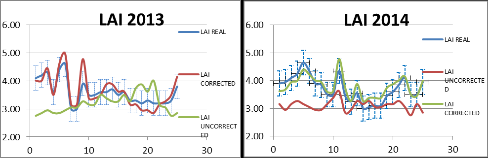
Vegetation indices were calculated using the spectrum range acquired from the spectroradiometric measurements. Figures 5, 6 and 7 show the values of radiometric, uncorrected and corrected from atmospheric effects NDVI, WDVI and LAI respectively.
In Figure 5, the reference value is the NDVI radiometric which are basically the real values of NDVI.
Standard Deviations taken from Table 4, for 2013 and 2014, are applied in the figure in the form of discontinue line (perpendicular blue line) above and below the values. This is done to configure the movement of the corresponding Uncorrected (red line) and Corrected values (green line). It is very obvious that NDVI uncorrected values or line do not follow the schematic sequence of the reference values (radiometric values) but has a rather significant different movement from point to point. Most of the cases are even out of the limit of the Standard deviation of real NDVI meaning that there is a basic difference. On the other hand, NDVI corrected values or line has almost identical way as the reference line. All the cases are included in the limits of real NDVI Standard Deviation identifying that there are no significant differences between real and uncorrected values for NDVI. This is the case for years, 2013 and 2014. On the other hand values of uncorrected NDVI seem to have significant differences from the real (radiometric) but also the corrected values of the NDVI. Most of the points are out of the Standard Deviation limits implying that if there is a relation this could not be sound.
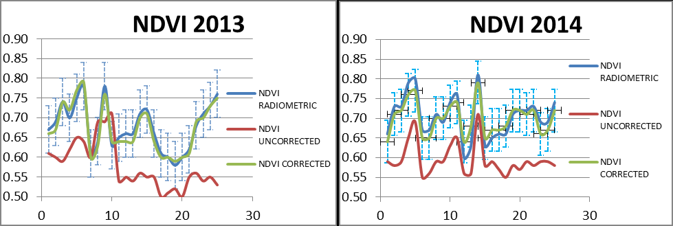
The same results come to light for the other two factors, WDVI and LAI. Uncorrected values of WDVI and LAI are differentiated from the reference (real) values or lines of the corresponding factors significantly and are out of the Standard Deviation’s limits for each factor, most of the times for the two years.
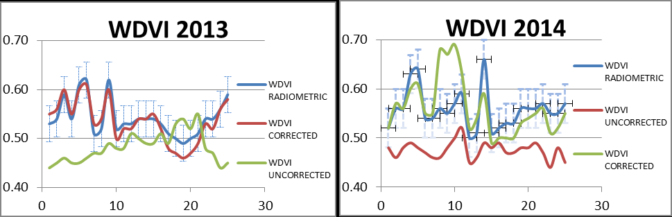
Corrected values are following the reference lines and are included in the Standard Deviation’s limits of each factor, except few single cases of WDVI 2014 and LAI 2013. Thus the general idea one receives from the specific figures and analysis is that uncorrected from atmospheric effects values have a significant difference from the real values while the corrected from atmospheric effects values are very close and within the limits of the real values’ Standard Deviation.
Figures 5-7 have provided a clue of the assumption raised by the authors that atmospheric effects have negative effect on the models using remotely sensed data. It has been shown that values from satellite images that have not undergone any atmospheric correction will have significant difference from the real values. Now intended purpose is to verify that statistically, and to illustrate that corrected from atmospheric effects values have no significant differences from the real values.
| T value | T statistical | Standard Error | Signifigance | ||||||||||||||||||||
|---|---|---|---|---|---|---|---|---|---|---|---|---|---|---|---|---|---|---|---|---|---|---|---|
| Relation | |||||||||||||||||||||||
| 2013 | 2014 | (n-1) d.f | 2013 | 2014 | 2013 | 2014 | |||||||||||||||||
| NDVI rad - NDVI corr. | 1.953 | 1.1 | 2.492 | 0.002 | 0.004 | 0.063 | 0.282 | ||||||||||||||||
| NDVI rad - NDVI uncorr. | 7.4 | 16.863 | 2.492 | 0.013 | 0.006 | 0 | 0 | ||||||||||||||||
| NDVI uncorr - NDVI corr. | 7.105 | -19.424 | 2.492 | 0.067 | 0.005 | 0 | 0 | ||||||||||||||||
| WDVI rad - WDVI corr. | 1.904 | -0.361 | 2.492 | 0.003 | 0.009 | 0.069 | 0.721 | ||||||||||||||||
| WDVI rad - WDVI uncorr. | 4.957 | 11.38 | 2.492 | 0.012 | 0.007 | 0 | 0 | ||||||||||||||||
| WDVI uncorr. - WDVI corr. | 3.863 | -8.02 | 2.492 | 0.014 | 0.101 | 0.001 | 0 | ||||||||||||||||
| LAI real - LAI corr. | 0.863 | -1.985 | 2.492 | 0.053 | 0.042 | 0.396 | 0.059 | ||||||||||||||||
| LAI real - LAI uncorr. | 2.888 | 6.572 | 2.492 | 0.135 | 0.09 | 0.008 | 0 | ||||||||||||||||
| LAI uncorr - LAI corr. | 2.631 | -9.688 | 2.492 | 0.165 | 0.07 | 0.015 | 0.000. |
Table 5: Student’s T-test for NDVI, WDVI and LAI. Paired couples of real-corrected, real-uncorrected and corrected- uncorrected v
Student’s t-test was applied based on the results (paired values) of the NDVI, WDVI and LAI for the two years. The results of the test are shown in Table 5.
SPSS statistical software was used to proceed with the statistical analysis and obtain the values of T-test to be compared with those of existing Statistical Tables for T- test shown at the third column of Table 5. The analysis has illustrated that the values of T observed between real values and corrected values of NDVI, WDVI and LAI were smaller than the Tstatistical, which implies that for (n-1) degrees of freedom and at a confidence level of 95%, these values do not have a significant statistical difference between them. Thus for all the cases where satellite images are atmospherically rectified there is not a statistically significant difference between the estimated (corrected) and measured (real) values.
In the case of comparing real NDVI, WDVI and LAI values to uncorrected values, the opposite phenomenon takes place, meaning that there is, in all cases, a statistically significant difference of the paired values, which means that uncorrected images cannot be used to After applying the Drum wheat prediction model yield values for 2013 and 2014 were retrieved. These values were compared graphically and statistically to real values in order to test the null hypothesis that if satellite images are not compensated for atmospheric correction then they cannot be used in crop yield modelling.
retrieve the corresponding NDVI, WDVI and LAI values since they will be misleading.
Crop Yield comparison
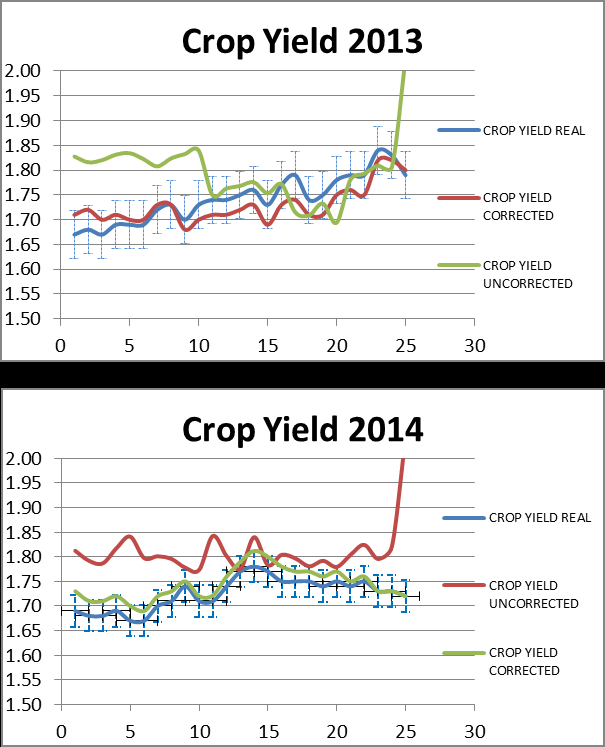
Figure 6, illustrates the real values of Crop Yield given from the Agricultural Research Institute of Cyprus for the specific plots which are considered to be the reference values. Standard Deviation of the specific values taken from Table 4, for 2013 and 2014 and applied in the figure in the form of discontinue line (perpendicular blue line) above and below the values.
This is done to configure the movement of the corresponding Uncorrected (green line) and Corrected values (red line). It is very obvious that Crop Yield uncorrected values or line do not follow the schematic sequence of the reference values (real values) but has a rather significant different movement from point to point. Most of the cases are even out of the limit of the Standard deviation of real values meaning that there is a basic difference. On the other hand Crop Yield corrected values or line has almost identical way as the reference line. All the cases are included in the limits of real values’ Standard Deviation identifying that there is no significant differences between real and uncorrected values. This is the case for years, 2013 and 2014.
Finally, Student’s t-test was applied based on the results (paired values) of the NDVI, WDVI and LAI for the two years. The results of the test are shown in Table 6.
| T value | T statistical | Standard Error | Signifigance | ||||||||||||||||||||
|---|---|---|---|---|---|---|---|---|---|---|---|---|---|---|---|---|---|---|---|---|---|---|---|
| Relation | |||||||||||||||||||||||
| 2013 | 2014 | (n-1) d.f | 2013 | 2014 | 2013 | 2014 | |||||||||||||||||
| CY real - CY corr. | 2.441 | 1.934 | 2.492 | 0.005 | 0.002 | 0.022 | 0.06 | ||||||||||||||||
| CY real - CY uncorr. | 3.164 | -6.757 | 2.492 | 0.017 | 0.012 | 0.004 | 0.002 | ||||||||||||||||
| CY uncorr. - CY corr. | 5.09 | 5.041 | 2.492 | 0.131 | 0.066 | 0 | 0.004 |
Table 6: Student’s T-test for Yield. Paired couples of real-corrected, real-uncorrected and corrected-uncorrected values.
The analysis has illustrated that the values of T observed between real values and corrected values of Crop Yield were smaller than the Tstatistical, which implies that for (n- 1) degrees of freedom and at a confidence level of 95%, these values do not have a significant statistical difference between them. Thus for all the cases where satellite images are atmospherically rectified there is not a statistically significant difference between the estimated (corrected) and measured (real) values.
In the case of comparing real Crop Yield values to uncorrected values, the opposite phenomenon takes place, meaning that there is, in all cases, a statistically significant difference of the paired values, which means that uncorrected images cannot be used to retrieve the corresponding NDVI, WDVI and LAI values since they will be misleading.
Conclusions
The purpose of the paper is to enlighten how atmospheric effects can affect Crop Yield Modelling when using remote sensing techniques. Since spatial factor is a trend, remotely sensed data is vital to support al sciences in solving theoretical and practical problems. But including such data in the ‘equation’ should be done correctly and avoid any bias such as atmospheric effects. The necessary atmospheric corrections to satellite images can have a significant influence on models using satellite images if not taken into account. An integrated effort to test the impact in all stages of Crop Yield modelling - vegetation indices, LAI and Crop Yield - has revealed the magnitude of atmospheric effects on Crop Yield on Durum wheat, using remote-sensing techniques.
It is very critical to apply atmospheric corrections to remove atmospheric effects from satellite images. If not, then the results could be misleading and cause severe problems, related to crop modelling generally. Results regarding Crop Yield show that omission or ineffective atmospheric corrections on Landsat 5TM,/7ETM+ satellite images always results to values that have a statistically significant difference Yield and may be misleading for policy makers. The paper aims to illustrate the importance of atmospheric effects removal from satellite images designated for model using remotely sensed data for predicting crop yield. This novel method has been developed in the Cyprus region, but since the local climate conditions resemble to the Mediterranean climatic conditions the method can be expanded also the Mediterranean region.
Conclusively, the trend of using satellite imagery for Crop Yield modelling is very important in agricultural management and has expanded all over the world the last decades. The use of satellite images provides the opportunity for monitoring yield on a systematic basis. Atmospheric effects have to be considered as very critical in this procedure, since they can cause severe deviations from the real values.
References
-
Milton EJ, Rollin EM, Emery DR (1995) Advances in field spectroscopy, Advances in Environmental Remote Sensing (ed. F.M. Danson and S.E. Plummer), John Wiley & Sons, Chichester.
-
Lawson M, Leavitt B, Rundquist D, Emanuel N, Perk R, et al. (2006) Compensating for irradiance fluxes when measuring the spectral reflectance of corals in-situ. GIScience & Remote Sensing 43(2): 111-127.
-
Dekker AG, Malthus TJ, Wijnen MM, Seyhan E (1992) The effect of spectral bandwidth and positioning on the spectral signature analysis of inland waters, Remote Sensing of Environment 41(2-3): 211-225.
-
D’Urso G, Belmonte AC 2006) Operative approaches to determine crop water requirements from Earth Observation data: methodologies and applications. AIP Conference Proceedings Naples 852(1): 14-25.
-
Hadjimitsis DG, Papadavid G, Kounoudes A (2008) Integrated method for monitoring irrigation demand in agricultural fields in Cyprus using satellite remote sensing and wireless sensor network. 4th International Conference on Information & Communication Technologies in Bio & Earth Sciences, Athens, Greece.
-
Papadavid G, Hadjimitsis D, Agapiou A (2009) Estimating Evapotranspiration using Remote Sensing Techniques for the sustainable use of irrigation water in Agriculture, 29th EARSeL Symposium, Chania, Crete.
-
Papadavid G, Hadjimitsis DG (2009) Spectral signature measurements during the whole life cycle of annual crops and sustainable irrigation management over Cyprus using remote sensing and spectro-radiometric data: the cases of spring potatoes and peas**.** Proc of SPIE 7472: 2.
-
Papadavid G, Agapiou A, Michaelides S, Hadjimitsis DG (2011) The integration of remote sensing and meteorological data for monitoring irrigation demand in Cyprus. Nat. Hazards earth syst. Sciences 9: 2009- 2014.
-
McCoy KR (1995) Resource Management information systems. Taylor and Francis, London, 244-281.
-
Atzberger C, Rembold F (2013) Mapping the Spatial Distribution of Winter Crops at Sub-Pixel Level Using AVHRR NDVI Time Series and Neural Nets. Remote Sensing 5(3): 1335-1354.
-
Atkinson PM, Jeganathan C, Dash J, Atzberger C (2012) Intercomparison of four models for smoothing satellite sensor timeseries data to estimate vegetation phenology. Remote Sens Environ 123: 400-417.
-
Meroni M, Atzberger C, Vancutsem C, Gobron N, Baret F, et al. (2013) A protocol for the evaluation of agreement between space remote sensing time series andapplication to SPOT-VEGETATION fAPAR products. International Journal of Applied Observations and Geoinformation 51: 1951-1962.
-
Quarmby NA, Milnes M, Hindle TL, Silleos N (1993) The use of multi-temporal NDVI measurements from AVHRR data for crop yield estimation and prediction. Int J Remote Sens 14(2): 199-210.
-
Balaghi R, Tychon B, Eerens H, Jlibene M (2008) Empirical regression models using NDVI, rainfall and temperature data for early prediction of wheat grain yields in Morocco. International Journal of Applied Earth Observation 10(4): 438-452.
-
Hayes MJ, Decker WL (1996) Using NOAA AVHRR data to estimate maize production in the United States Corn Belt. Int J Remote Sens 17(16): 3189- 3200.
-
Papadavid G, Hadjimitsis D (2014) An image based method for crop yield prediction using remotely sensed and crop canopy data: the case of Paphos district, western Cyprus. Proc SPIE 9229, Second International Conference on Remote Sensing and Geoinformation of the Environment (RSCy2014).
-
Duggin MJ, Piwinski D (1984) Recorded radiance indices for vegetation monitoring using NOAA AVHRR data; atmospheric and other effects in multitemporal data sets. Appl Optics 23(15): 2620-2623.
-
Honkavaara E, Arbiol R, Markelin L, Martinez L, Cramer M, et al. (2009) Digital airborne photogrammetry-A new tool for quantitative remote sensing?-A state-of-the-art review on radiometric aspects of digital photogrammetric images. Remote Sens 1(3): 577-605.
-
Bagheri S (2011) Nearshore water quality estimation using atmospherically corrected AVIRIS data. Remote Sens 3(2): 257-269.
-
Song C, Woodcock EC (2003) Monitoring forest succession with multitemporal Landsat images: Factors of uncertainty. IEEE Trans Geosci Remote Sens 41(11): 2557-2567.
-
Valipour M (2012) A comparison between horizontal and vertical drainage systems (include pipe drainage, open ditch drainage, and pumped wells) in anisotropic soils. IOSR J Mech Civil Eng 4(1): 7-12.
-
Valipour M (2012) Ability of Box-Jenkins models to estimate of reference potential evapotranspiration (A case study: Mehrabad Synoptic Station, Tehran, Iran). IOSR Journal of Agriculture and Veterinary Science (IOSR-JAVS) 1(5): 1-11.
-
Valipour M (2012) Hydro-module determination for vanaei village in Eslam Abad Gharb, Iran. ARPN J Agric Biol Sci 7(12): 968-976.
-
Valipour M (2013) Use of surface water supply index to assessing of water resources management in Colorado and Oregon, US.
-
Valipour M (2013) Increasing irrigation efficiency by management strategies: cutback and surge irrigation. ARPN Journal of Agricultural and Biological Science 8(1): 35-43.
-
Valipour M (2014) Analysis of potential evapotranspiration using limited weather data. Applied Water Science 7(1): 187-197.
-
Valipour M (2014) Application of new mass transfer formulae for computation of evapotranspiration. Journal of Applied Water Engineering and Research 2(1): 33-46.
-
Valipour M (2016) How Much Meteorological Information Is Necessary to Achieve Reliable Accuracy for Rainfall Estimations? Agriculture 6(4): 53.
-
Che N Price JC (1992) Survey of Radiometric calibration results and methods for visible and near infrared channels of NOAA-7, -9, and -11 AVHRRs. Remote Sens. Environ 4(1): 19-27.
-
Hadjimitsis DG, Papadavid G, Agapiou A, Themistocleous K, Hadjimitsis MG, et al. (2010) Atmospheric correction for satellite remotely sensed data intended for agricultural applications: Impact on vegetation indices. Natural Hazards Earth Syst Sci 10: 89-95.
-
Bastiaanssen WGM, Molden DJ, Makin IW (2000) Remote sensing for irrigated agriculture: Examples from research and possible applications. Agr Water Manage 46(2): 137-155.
-
Kaufman YJ, Sendra C (1988) Algorithm for automatic atmospheric corrections to visible and near-IR satellite imagery. Int J Remote Sens 9(8): 1357-1381.
-
Courault D, Seguin B, Olioso A (2003) Review to Estimate Evapotranspiration from Remote Sensing Data: Some Examples from the Simplified Relationship to the Use of Mesoscale Atmospheric Models. ICID International Workshop on Remote Sensing of ET for Large Regions, Montpellier, France.
-
Hadjimitsis DG, Clayton CRI, Hope VS (2004) An assessment of the effectiveness of atmospheric correction algorithms through the remote sensing of some reservoirs. Int J Remote Sens 25(18): 3651- 3674.
-
Hadjimitsis DG, Clayton CRI, Hope VS (2011) The Importance of Accounting for Atmospheric Effects in Satellite Remote Sensing: A Case Study from the Lower Thames Valley Area, UK. The Seventh International Conference and Exposition on Engineering, Construction, Operations, and Business in Space. ASCE Conference on Space and Robotics, Albuquerque, NM, USA.
-
Hadjimitsis DG, Clayton CRI, Retalis A (2004) On the darkest pixel atmospheric correction algorithm: a revised procedure applied over satellite remotely sensed images intended for environmental applications. Remote Sensing for Environmental Monitoring, Proc SPIE 5239: 464-471.
-
Papadavid G, Hadjimitsis DG, Perdikou S, Michaelides S, Toulios L, et al. (2011) Use of field spectroscopy for exploring the impact of atmospheric effects on Landsat 5 TM / 7 ETM+ satellite images intended for hydrological purposes in Cyprus. GIScience and Remote Sensing 48(2): 280-298.
-
Hadjimitsis DG, Papadavid G, Agapiou A, Themistocleous K, Hadjimitsis MG, et al. (2010) Atmospheric correction for satellite remotely sensed data intended for agricultural applications: impact on vegetation indices. Nat Hazards earth syst. Sciences 10: 89-95.
-
Hadjimitsis DG, Clayton CRI, Retalis A (2009) The use of selected pseudo-invariant targets for the application of atmospheric correction in multi- temporal studies using satellite remotely sensed imagery. International Journal of Applied Earth Observation and Geoinformation 11(3): 192-200.
-
Hadjimitsis DG, Clayton CRI, Hope VS (2004) An assessment of the effectiveness of atmospheric correction algorithms through the remote sensing of some reservoirs. International Journal of Remote Sensing, 25(18): 3651-3674.
-
Duanjun Lu, Jie Song (2004) A Simplified Atmospheric Correction Procedure for Estimating Surface Temperature from AVHRR Thermal Data. GIScience & Remote Sensing 41(1): 81-94.
-
Milton EJ (1987) Review Article Principles of field spectroscopy. International Journal of Remote Sensing 8(12): 1807-1827.
-
D’Urso G, Menenti M 1995) Mapping crop coefficients in irrigated areas from Landsat TM images; Proceed. European Symposium on Satellite Remote Sensing II, Europto, Paris, sett.’95; SPIE, Intern Soc Optical Engineering 2585: 41-47Bowman.
-
Brunsell NA, Pontes PPB, Lamparelli RAC (2009) Remotely sensed phenology of coffee and its relationship to yield. GI Science & Remote Sensing 46(3): 289-304.
-
Milton EJ, Schaepman ME, Anderson K, Kneubuhler M, Fox N (2009) Progress in Field Spectroscopy. Remote Sensing of Environment 113(Supply 1): S92-S109.
-
Bouman BAM, van Kasteren HWJ, Uenk D (1992) Standard Relations to Estimate Ground Cover and LAI of Agricultural Crops from Reflectance Measurements. Europ J Agronomy 1(4): 249-262.
-
Stancalie G, Nertan A, Toulios L (2010) Satellite based methods for the estimation of Leaf Area Index. Toulios L, Stancalie G (Eds.), Satellite data availability, methods and challenges for the assessment of climate change and variability impacts on agriculture. Emm Lavdakis OE publishers, Larissa, Greece, pp: 49-74.
-
Lambert R, Peeters A, Toussaint B (1999) LAI evolution of perennial ryegrass crop estimated from the sum of temperatures in spring time. Agric Forest Meteo 97(1): 1-8.
- Enhancement of Vegetative Growth and Fruit Yield in Cucumber (Cucumis sativus L.) via Spiritual Blessing (Biofield) Energy Intervention
- Production of Açaí (Euterpe oleracea Mart.) under Different Agroforestry System Management Intensities in Amazonian Floodplain (Varzea) Forests
- Coffee and the Production Region: What is the Secret to the Expression "Quality"?
- Experiential Agripreneurship Training in Sub-Saharan Africa: Integrating a Business Incubator into Postgraduate Livestock Education at the University of Buea
- Advances in Agricultural High-Quality Development
- Linking Compost Residue to ABAGE in Plants - a Short Note