Assessment of Eco-Environment Quality of Darjeeling and Kalimpong Districts, West Bengal, India using Remote Sensing based Ecological Index
Ecological Environmental Quality (EEQ) is an important measure of evaluating the comprehensive characteristics of ecosystem elements, structure, and function that can reflect the strengths and weaknesses of the regional ecological environment. In the present study, an attempt has been made to assess the Eco-Environment Quality (EEQ) and its spatio-temporal changes in Darjeeling and Kalimpong districts using Remote Sensing based Ecological Index (RSEI) during the years 1999 and 2022. It is assessed by synthesizing four ecological indicators viz. Normalized Difference Vegetation Index (NDVI), Normalized Difference Built-up and Bare Soil Index (NDBSI), Land Surface Moisture (LSM), and Land Surface Temperature (LST) representing greenness, dryness, wetness, and heat. Further, Principal Component Analysis (PCA) is performed within the Pressure- State-Response (PSR) Framework, where NDBSI is put under the “Pressure” category, NDVI under “State” and “LSM” & “LST” under the “Response” category. The results indicate that mean RSEI values have increased from 0.49 in 1999 to 0.58 in 2022, showing an overall improvement of 15% in ecological environment quality during the study period. The spatial distribution of ecological indicators shows that the northern part of the study area (part of Darjeeling Himalaya) has relatively higher values in case of NDVI and LSM which indicates better ecological quality; while the southern region which is the plain area shows relatively higher values in case of NDBSI and LST, indicating poor ecological quality of the region.
Abbreviations
EEQ: Ecological Environmental Quality; PCA: Principal Component Analysis; PSR: Pressure-State-Response; RSEI: Remote Sensing based Ecological Index; LSM: Land Surface Moisture; TCT: Tasselled Cap Transformation; TOA: Top of Atmosphere.
Introduction
The ecological environment (EE) is a natural-economic- social complex ecosystem. A good EE plays a vital role in promoting social stability, ecological security, and sustainable development. It represents the stability and resilience of the ecosystem, depicting an inter-relationship between humans and nature [1]. Excessive exploitation of natural resources and intense human activities such as rapid urbanization, unplanned development, uncontrolled industrialization etc. have severely degraded the eco-environment causing threat to sustained socio-economic development and survival of mankind. These changes can have negative impacts on both the health of ecosystems and the well-being of the resident [2]. Therefore, researchers are paying attention on quantifying the ecological change emerging from global climate change and depletion of resources by anthropogenic actions [3].
Ecological Environmental Quality (EEQ) is an important measure of evaluating the comprehensive characteristics of ecosystem elements, structure and function that can reflect the strengths and weaknesses of regional ecological environment. Presently many studies on EEQ are being carried out at global, regional and local scale using Remote Sensing and GIS techniques [4, 5, 6]. Remote sensing has a distinct advantage of providing real time in-situ precise data at different scales and resolutions from which ecological indicators can be comprehensively identified using the wide range of spectral information [7]. Several remote sensing- based indices were created to monitor ecological state of a region. For example, Normalized Difference Vegetation Index (NDVI), Normalized Difference Built-up Index (NDBI), Land Surface Temperature (LST) for heat island effect analysis, or ecosystem services value, etc and methods are developed to quantify and map ecosystem functions [8, 9, 10, 11]. However, most of these methods and indices focus solely on a particular feature of an ecosystem not considering the complex forces including human interactions that affect the quality and structure of the ecosystem. Consequently they are unable to adequately establish the strengths and weaknesses of the ecological environment and provide objective outcomes [12].
Compared to these indices, Remote Sensing based Ecological Index (RSEI) provides a well-suited quantitative assessment of ecological quality monitoring at different periods [1]. The RSEI has been applied in various studies to evaluate ecological conditions in different regions of the world. Xu HQ, et al. have proposed the Remote Sensing based Ecological Index (RSEI) by integrating four indicators (greenness, wetness, dryness and heat) using Principal Component Analysis (PCA) for the assessment of ecological conditions in Fuzhou City, China [7]. Philip, et al. [1] has evaluated ecological quality of Akkulam-Veli Lake Basin, in Thiruvananthapuram, Kerala using Remote-Sensing Ecological Index (RSEI) and an overall deterioration in ecological quality is observed during the study period with the RSEI value of 0.733 in 2000 to 0.611 in 2023. Wang, et al. has evaluated the spatio-temporal changes in ecological quality in East China during 2000-2020 and results showed an decreasing and increasing trend in mean RSEI values. Low values are mainly associated with densely populated areas, due to having an imprint of human activities. On the other hand, a study by Xu H, et al. [13] has revealed an ecological improvement in Fujian province, China during the period 2002-2017 as a result of rise in mean RSEI scores due to increase in forest areas. Therefore, RSEI model provides comparatively a new comprehensive method for assessing ecological environmental quality based on entirely remote sensing data [12, 13].
In the present study we have selected Darjeeling and Kalimpong Districts in West Bengal to evaluate the ecological status using RSEI model within Pressure-State-Response (PSR) Framework. This PSR framework is used to segregate and explain the remote sensing indices under the Pressure, State and Response categories. Being a part of Eastern Himalayan Ecosystem, Darjeeling has a wide range of renewable and non-renewable resources. Since the arrival of Britishers during nineteenth century, the physico-cultural set up of the region has been interrupted to a certain extent. In case of Darjeeling Himalaya or Darjeeling district as a whole, there are studies focusing on environmental degradation of Darjeeling hilly areas [14]; urbanization and associated problems in North Bengal [15]; history of urbanization in Darjeeling in the 19th century [16]; constraints in sustainable urban development in Darjeeling [17] etc. Spatio-temporal urban expansion and land use land cover change over the municipal areas of Darjeeling such Siliguri, Mirik is also been analysed [18, 19, 20]. Most of the researches have discussed about urbanization, its impact on environment and other associated issues but a comprehensive assessment to understand the ecological change due to human activities is untouched yet in Darjeeling. Extensive deforestation, unplanned construction of settlements and roads, irrational and unscientific mining, improper drainage system has led to the environmental degradation as a whole . Changes in land use from natural vegetation to tea plantation, agriculture and settlements have intensified in last few decades. Extensive livestock grazing has become another source of biodiversity loss, which breaks the rhythm of natural ecosystem. It is reported that Darjeeling town is facing continuous conflict among economic, environmental and social sustainability due to lack of investment in infrastructure and service provisions. Therefore, sustainability of the landscape is being questioned. These activities are posing serious threats to the ecosystem at local level, which are irreversible damage for the biodiversity. So, it is necessary to check the environmental quality of Darjeeling from ecological perspective. Therefore, to answer the query related to environmental quality, present study aims at (1) finding out the spatio-temporal distribution of ecological indicators over Darjeeling and Kalimpong Districts in 1999 and 2022, (2) assessing the ecological change over the study area during the same time frame under study, and (3) evaluating the current ecological conditions of the region using RSEI model. Present study thus can contribute in the regional development by quantifying the ecological change in last 20 years. The outcome of this research will contribute in understanding the regional ecological changes over last two decades.
Materials and Methods
Study Area
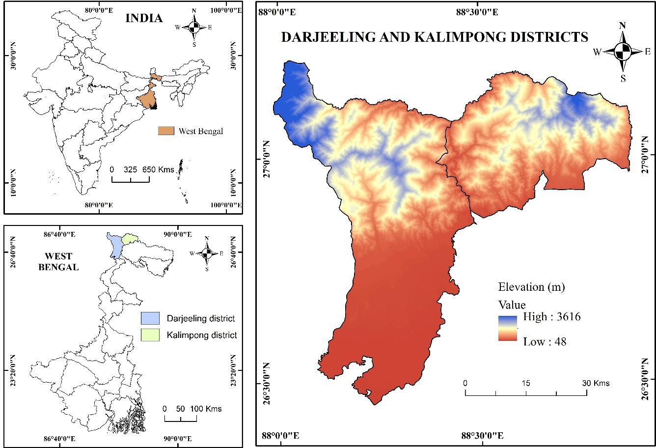
Darjeeling, located between 26°31´N-27°13´N latitude and 87°59´E-88°53´E, longitudes having 3149 sq.km area (as per 2011 census) is the northern most district of West Bengal. It consists of four sub-divisions i.e., Darjeeling, Kalimpong, Kurseong, and Siliguri. In the year of 2017, Kalimpong sub- division was declared as a separate district. Therefore, the new sub-divisions after 2017 are Darjeeling Sadar, Kurseong, Siliguri, and Mirik. The central attraction, principal town and administrative headquarter of the region is Darjeeling town, which has an area of nearly 10.75 sq.km. Geographically the district has two major divisions, hills in the north and plains in the south. The hills varying in elevation from 400 to 3,000 metres rise abruptly from the plains with a north-west to south-east alignment (Figure 1). They are part of lower or Shivalik Himalayas characterised by ridges, bold spurs, and narrow deep valleys. The plains with an average elevation of
80 to 300 meters lying in the south are marshy low-lying area called Terai. The district is drained by Teesta, Mahananda, Jaldhaka, Balason, Mechi, Rangeet, and Rammam rivers [21]. It has temperate subtropical highland climate (Köppen climate classification: Cwb). The maximum temperature reaches up to 24°C-27°C during summer and 14°C-17°C in winter, while minimum temperature ranges between 16°C-19°C and 5°C-6°C in summer and winter respectively. It receives an average annual rainfall of 220 cm per year, ranging from 1 inch in December-January to 34 inches in July-August.
Most of the ridges and valleys in Darjeeling hills are dominated by forest cover, and in many cases, they are altered into tea estates and other cultivated lands. For being a famous tourist spot in West Bengal, Darjeeling Himalaya has relatively high population density. Due to limitations in extending agricultural land, the forested and protected areas are getting encroached to meet the increasing population pressure on hills. Conversion of forest and grass lands into agriculture and settlements are mostly common in Darjeeling. Thus, changes in land use are leaving imprints on the ecology of the area. Hence, the assessment on regional ecological change can be a good example for understanding the ecological status of the region.
Database
This study is based on Landsat images (Table 1) downloaded freely from USGS (United States Geological Survey) website (https://earthexplorer.usgs.gov/) using Earth Explorer. These images were geometrically corrected and reprojected into WGS 1984 UTM Zone 45 in GIS environment.
| Sensor | Path/Row | Year | Spatial Resolution |
|---|---|---|---|
| Landsat 5 TM | 139/41 & 139/42 | 3rd March 1999 | 30 meters |
| Landsat 9 OLI/TIRS | 139/41 & 139/42 | 10th March 2022 | 30 meters |
Table 1: Details of Landsat data used.
Methodology
The Ecological Environmental Quality (EEQ) of the study $$ \mathrm {E} = \sum_ {i = 1} ^ {n} \mathrm {E} _ {i} = \sum_ {i = 1} ^ {n} \mathrm {E} _ {i} = \sum_ {i = 1} ^ {n} \mathrm {E} _ {i} = \sum_ {i = 1} ^ {n} \mathrm {E} _ {i} = \sum_ {i = 1} ^ {n} \mathrm {E} _ {i} = \sum_ {i = 1} ^ {n} \mathrm {E} _ {i} = \mathrm {E} _ {i} = \mathrm {E} _ {i} = \mathrm {E} _ {i} = \mathrm {E} _ {i} = \mathrm {E} _ {i} = \mathrm {E} _ {i} = \mathrm {E} _ {i} = \mathrm {E} _ {i} = \mathrm {E} _ {i} = \mathrm {E} _ {i} = \mathrm {E} _ {i} = \mathrm {E} _ {i} = \mathrm {E} _ {i} = \mathrm {E} _ {i} = \mathrm {E} _ {i} = \mathrm {E} _ {i} = \mathrm {E} _ {i} = \mathrm {E} _ {i} = \mathrm {E} _ {i} = \mathrm {E} _ {i} = \mathrm {E} _ {i} = \mathrm {E} _ {i} = \mathrm {E} _ {i} = \mathrm {E} _ {i} = \mathrm {E} _ {i} = \mathrm {E} _ {i} = \mathrm {E} _ {i} = \mathrm {E} _ {i} = \mathrm {E} _ {i} = \mathrm {E} _ {i} = \mathrm {E} _ {i} = \mathrm {E} _ {i} = \mathrm {E} _ {i} = \mathrm {E} _ {i} = \mathrm {E} _ {i} = \mathrm {E} _ {i} = \mathrm {E} $$
\mathrm {E} = \frac {1}{2} \mathrm {A} ^ {2} + \frac {1}{2} \mathrm {B} ^ {2} + \frac {1}{2} \mathrm {C} ^ {2}
$$ $$
\mathrm {E} = \frac {1}{2} \mathrm {A} ^ {2} + \frac {1}{2} \mathrm {B} ^ {2}
$$ $$
\mathrm {E} = \frac {1}{2} \mathrm {A} ^ {2} + \mathrm {B} ^ {2}
$$ $$
\mathrm {E} = \frac {1}{2} \mathrm {A} ^ {2} + \mathrm {B} ^ {2}
$$ $$
\mathrm {E} = \frac {1}{2} \mathrm {A} ^ {2} + \mathrm {B} ^ {2}
$$ $$
\mathrm {E} = \frac {1}{2} \mathrm {A} ^ {2} + \mathrm {B} ^ {2}
$$ $$
\mathrm {E} = \mathrm {E} {1} + \mathrm {E} {2} + \dots + \mathrm {E} _ {n}
$$ $$
\mathrm {E} = \frac {1}{2} \mathrm {A} ^ {2} + \mathrm {B} ^ {2}
$$ $$
\mathrm {E} = \frac {1}{2} \mathrm {A} ^ {2} + \frac {1}{2} \mathrm {B} ^ {2} + \frac {1}{2} \mathrm {C} ^ {2}
$$ $$
\mathrm {E} = \frac {1}{2} \mathrm {A} ^ {2} + \frac {1}{2} \mathrm {B} ^ {2} + \frac {1}{2} \mathrm {C} ^ {2}
$$ $$
\mathrm {E} = \frac {1}{2} \mathrm {A} ^ {2} + \mathrm {B} ^ {2}
$$ $$
\mathrm {E} = \frac {1}{2} \mathrm {A} ^ {2} + \mathrm {B} ^ {2}
$$ $$
\mathrm {E} = \frac {1}{2} \mathrm {A} ^ {2} + \frac {1}{2} \mathrm {B} ^ {2} + \frac {1}{2} \mathrm {C} ^ {2}
$$ $$
\mathrm {E} = \frac {1}{2} \mathrm {A} ^ {2} + \mathrm {B} ^ {2}
$$ $$
\mathrm {E} = \mathrm {E} {1} + \mathrm {E} {2} + \dots + \mathrm {E} _ {n}
$$ $$
\mathrm {E} = \frac {1}{2} \mathrm {A} ^ {2} + \mathrm {B} ^ {2}
$$ $$
\mathrm {E} = \frac {1}{2} \mathrm {A} ^ {2} + \frac {1}{2} \mathrm {B} ^ {2} + \frac {1}{2} \mathrm {C} ^ {2}
$$ $$
\mathrm {E} = \frac {1}{2} \mathrm {A} ^ {2} + \frac {1}{2} \mathrm {B} ^ {2} + \frac {1}{2} \mathrm {C} ^ {2}
$$ $$
\mathrm {E} = \frac {1}{2} \mathrm {A} ^ {2} + \frac {1}{2} \mathrm {B} ^ {2} + \frac {1}{2} \mathrm {C} ^ {2}
$$ $$
\mathrm {E} = \frac {1}{2} \mathrm {A} ^ {2} + \frac {1}{2} \mathrm {B} ^ {2} + \frac {1}{2} \mathrm {C} ^ {2}
$$ $$
\mathrm {E} = \frac {1}{2} \mathrm {A} ^ {2} + \mathrm {B} ^ {2}
$$ $$
\mathrm {E} = \frac {1}{2} \mathrm {A} ^ {2} + \mathrm {B} ^ {2}
$$ $$
\mathrm {E} = \frac {1}{2} \mathrm {A} ^ {2} + \mathrm {B} ^ {2}
$$ $$
\mathrm {E} = \frac {1}{2} \mathrm {A} ^ {2} + \mathrm {B} ^ {2}
$$ $$
\mathrm {E} = \frac {1}{2} \mathrm {A} ^ {2} + \mathrm {B} ^ {2}
$$ $$
\mathrm {E} = \frac {1}{2} \mathrm {A} ^ {2} + \mathrm {B} ^ {2}
$$ $$
\mathrm {E} = \frac {1}{2} \mathrm {A} ^ {2} + \mathrm {B} ^ {2}
$$ $$
\mathrm {E} = \frac {1}{2} \mathrm {A} ^ {2} + \mathrm {B} ^ {2}
$$ $$
\mathrm {E} = \mathrm {E} {1} + \mathrm {E} {2} + \dots + \mathrm {E} _ {n}
$$ $$
\mathrm {E} = \frac {1}{2} \mathrm {A} ^ {2} + \mathrm {B} ^ {2}
$$ $$
\mathrm {E} = \frac {1}{2} \mathrm {A} ^ {2} + \frac {1}{2} \mathrm {B} ^ {2}
$$ $$
\mathrm {E} = \frac {1}{2} \mathrm {A} ^ {2} + \frac {1}{2} \mathrm {B} ^ {2} + \frac {1}{2} \mathrm {C} ^ {2}
$$ $$
\mathrm {E} = \frac {1}{2} \mathrm {A} ^ {2} + \mathrm {B} ^ {2}
$$ $$
\mathrm {E} = \frac {1}{2} \mathrm {A} ^ {2} + \frac {1}{2} \mathrm {B} ^ {2} + \frac {1}{2} \mathrm {C} ^ {2}
$$ $$
\mathrm {E} = \frac {1}{2} \mathrm {A} ^ {2} + \mathrm {B} ^ {2}
$$ $$
\mathrm {E} = \frac {1}{2} \mathrm {A} ^ {2} + \mathrm {B} ^ {2}
$$ $$
\mathrm {E} = \mathrm {E} {1} + \mathrm {E} {2} + \dots + \mathrm {E} _ {n}
$$ $$
\mathrm {E} = \frac {1}{2} \mathrm {A} ^ {2} + \frac {1}{2} \mathrm {B} ^ {2}
$$ $$
\mathrm {E} = \frac {1}{2} \mathrm {A} ^ {2} + \frac {1}{2} \mathrm {B} ^ {2} + \frac {1}{2} \mathrm {C} ^ {2}
$$ $$
\mathrm {E} = \frac {1}{2} \mathrm {A} ^ {2} + \frac {1}{2} \mathrm {B} ^ {2}
$$ $$
\mathrm {E} = \frac {1}{2} \mathrm {A} ^ {2} + \frac {1}{2} \mathrm {B} ^ {2} + \frac {1}{2} \mathrm {C} ^ {2}
$$ $$
\mathrm {E} = \frac {1}{2} \mathrm {A} ^ {2} + \frac {1}{2} \mathrm {B} ^ {2} + \frac {1}{2} \mathrm {C} ^ {2}
$$ $$
\mathrm {E} = \frac {1}{2} \mathrm {A} ^ {2} + \mathrm {B} ^ {2}
$$ $$
\mathrm {E} = \frac {1}{2} \mathrm {A} ^ {2} + \frac {1}{2} \mathrm {B} ^ {2} + \frac {1}{2} \mathrm {C} ^ {2}
$$ $$
\mathrm {E} = \frac {1}{2} \mathrm {A} ^ {2} + \frac {1}{2} \mathrm {B} ^ {2}
$$ $$
\mathrm {E} = \frac {1}{2} \mathrm {A} ^ {2} + \mathrm {B} ^ {2} + \mathrm {C} ^ {2} + \mathrm {D} ^ {2} + \mathrm {E} ^ {2}
$$ $$
\mathrm {E} = \frac {1}{2} \mathrm {A} ^ {2} + \frac {1}{2} \mathrm {B} ^ {2} + \frac {1}{2} \mathrm {C} ^ {2}
$$ $$
\mathrm {E} = \frac {1}{2} \mathrm {A} ^ {2} + \mathrm {B} ^ {2}
$$ $$
\mathrm {E} = \mathrm {E} {1} + \mathrm {E} {2} + \dots + \mathrm {E} _ {n}
$$ $$
\mathrm {E} = \frac {1}{2} \mathrm {A} ^ {2} + \mathrm {B} ^ {2}
$$ $$
\mathrm {E} = \frac {1}{2} \mathrm {A} ^ {2} + \mathrm {B} ^ {2}
$$ $$
\mathrm {E} = \frac {1}{2} \mathrm {A} ^ {2} + \mathrm {B} ^ {2}
$$ $$
\mathrm {E} = \mathrm {E} {1} + \mathrm {E} {2} + \dots + \mathrm {E} _ {n}
$$ $$
\mathrm {E} = \frac {1}{2} \mathrm {A} ^ {2} + \mathrm {B} ^ {2}
$$ $$
\mathrm {E} = \frac {1}{2} \mathrm {A} ^ {2} + \mathrm {B} ^ {2} + \mathrm {C} ^ {2} + \mathrm {D} ^ {2} + \mathrm {E} ^ {2} + \mathrm {F} ^ {2} + \mathrm {G} ^ {2} + \mathrm {H} ^ {2} + \mathrm {I} ^ {2} + \mathrm {J} ^ {2} + \mathrm {K} ^ {2} + \mathrm {L} ^ {2} + \mathrm {M} ^ {2} + \mathrm {N} ^ {2} + \mathrm {O} ^ {2} + \mathrm {P} ^ {2} + \mathrm {Q} ^ {2} + \mathrm {R} ^ {2} + \mathrm {S} ^ {2} + \mathrm {T} ^ {2} + \mathrm {U} ^ {2} + \mathrm {V} ^ {2} + \mathrm {W} ^ {2} + \mathrm {X} ^ {2} + \mathrm {Y} ^ {2} + \mathrm {Z} ^ {2}
$$ $$
\mathrm {E} = \frac {1}{2} \mathrm {A} ^ {2} + \frac {1}{2} \mathrm {B} ^ {2} + \frac {1}{2} \mathrm {C} ^ {2}
$$ $$
\mathrm {E} = \frac {1}{2} \mathrm {A} ^ {2} + \mathrm {B} ^ {2}
$$ $$
\mathrm {E} = \frac {1}{2} \mathrm {A} ^ {2} + \frac {1}{2} \mathrm {B} ^ {2} + \frac {1}{2} \mathrm {C} ^ {2}
$$ $$
\mathrm {E} = \frac {1}{2} \mathrm {A} ^ {2} + \frac {1}{2} \mathrm {B} ^ {2} + \frac {1}{2} \mathrm {C} ^ {2}
$$ Figure 2: Methodological workflow of the study.
Generation of Remote Sensing based Ecological Index (RSEI)
Water, vegetation and temperature are the major factors that affect the environment. Therefore, dryness, greenness, wetness and heat are the major parameters to study the status of environment. Dryness refers to build-induced land- area is evaluated using RSEI model and the indicators of RSEI are explained within the Pressure-State-Response (PSR) framework (Figure 2).
$$ \mathrm {E} = \frac {1}{2} \mathrm {A} ^ {2} + \frac {1}{2} \mathrm {B} ^ {2} $$ $$ \mathrm {E} = \frac {1}{2} \mathrm {A} ^ {2} + \mathrm {B} ^ {2} $$ $$ \mathrm {E} = \frac {1}{2} \mathrm {A} ^ {2} + \mathrm {B} ^ {2} $$ $$ \mathrm {E} = \frac {1}{2} \mathrm {A} ^ {2} + \mathrm {B} ^ {2} $$ $$ \mathrm {E} = \frac {1}{2} \mathrm {A} ^ {2} + \frac {1}{2} \mathrm {B} ^ {2} $$ $$ \mathrm {E} = \mathrm {E} _ {1} + \mathrm {E} _ {2} + \dots + \mathrm {E} _ {n} $$ $$ \mathrm {E} = \frac {1}{2} \mathrm {A} ^ {2} + \mathrm {B} ^ {2} $$
$$ \mathrm {E} = \frac {1}{2} \mathrm {A} ^ {2} + \mathrm {B} ^ {2} $$
$$ \mathrm {E} = \frac {1}{2} \mathrm {A} ^ {2} + \mathrm {B} ^ {2} $$
$$ \mathrm {E} = \frac {1}{2} \mathrm {A} ^ {2} + \mathrm {B} ^ {2} $$
$$ \mathrm {E} = \frac {1}{2} \mathrm {A} ^ {2} + \frac {1}{2} \mathrm {B} ^ {2} $$ $$ \mathrm {E} = \frac {1}{2} \mathrm {A} ^ {2} + \mathrm {B} ^ {2} $$ $$ \mathrm {E} = \frac {1}{2} \mathrm {A} ^ {2} + \mathrm {B} ^ {2} $$ $$ \mathrm {E} = \frac {1}{2} \mathrm {A} ^ {2} + \mathrm {B} ^ {2} $$ $$ \mathrm {E} = \frac {1}{2} \mathrm {A} ^ {2} + \mathrm {B} ^ {2} $$ $$ \mathrm {E} = \frac {1}{2} \mathrm {A} ^ {2} + \frac {1}{2} \mathrm {B} ^ {2} + \frac {1}{2} \mathrm {C} ^ {2} $$ $$ \mathrm {E} = \frac {1}{2} \mathrm {A} ^ {2} + \mathrm {B} ^ {2} $$ $$ \mathrm {E} = \frac {1}{2} \mathrm {A} ^ {2} + \mathrm {B} ^ {2} $$ $$ \mathrm {E} = \frac {1}{2} \mathrm {A} ^ {2} + \mathrm {B} ^ {2} $$ $$ \mathrm {E} = \mathrm {E} _ {1} + \mathrm {E} _ {2} + \dots + \mathrm {E} _ {n} $$ $$ \mathrm {E} = \frac {1}{2} \mathrm {A} ^ {2} + \mathrm {B} ^ {2} $$ $$ \mathrm {E} = \frac {1}{2} \mathrm {A} ^ {2} + \mathrm {B} ^ {2} $$ $$ \mathrm {E} = \mathrm {E} _ {1} + \mathrm {E} _ {2} + \dots + \mathrm {E} _ {n} $$ $$ \mathrm {E} = \frac {1}{2} \mathrm {A} ^ {2} + \mathrm {B} ^ {2} $$ $$ \mathrm {E} = \frac {1}{2} \mathrm {A} ^ {2} + \frac {1}{2} \mathrm {B} ^ {2} + \frac {1}{2} \mathrm {C} ^ {2} $$ $$ \mathrm {E} = \mathrm {E} _ {1} + \mathrm {E} _ {2} + \dots + \mathrm {E} _ {n} $$ $$ \mathrm {E} = \frac {1}{2} \mathrm {A} ^ {2} + \mathrm {B} ^ {2} $$ $$ \mathrm {E} = \frac {1}{2} \mathrm {A} ^ {2} + \mathrm {B} ^ {2} $$ $$ \mathrm {E} = \frac {1}{2} \mathrm {A} ^ {2} + \mathrm {B} ^ {2} $$ $$ \mathrm {E} = \frac {1}{2} \mathrm {A} ^ {2} + \mathrm {B} ^ {2} $$ $$ \mathrm {E} = \mathrm {E} _ {1} + \mathrm {E} _ {2} + \dots + \mathrm {E} _ {n} $$ $$ \mathrm {E} = \frac {1}{2} \mathrm {A} ^ {2} + \mathrm {B} ^ {2} $$ $$ \mathrm {E} = \frac {1}{2} \mathrm {A} ^ {2} + \frac {1}{2} \mathrm {B} ^ {2} $$ $$ \mathrm {E} = \frac {1}{2} \mathrm {A} ^ {2} + \mathrm {B} ^ {2} $$ $$ \mathrm {E} = \frac {1}{2} \mathrm {A} ^ {2} + \frac {1}{2} \mathrm {B} ^ {2} $$ surface desiccation, greenness to the state of vegetation cover, wetness represents moisture condition and heat to changing temperature and climatic conditions. RSEI combines these four indicators to detect the ecological condition of a region. These indicators are first calculated individually and then integrated to obtain the synthetic value of RSEI. This is done using the ecological indices derived from Landsat data (Table
1) at the pixel level as discussed below:
**Calculation of Indicators**
Dryness
It is assessed using Normalised Difference Built-up and Bare Soil Index (NDBSI) using Equations 1-3. It is a proxy of "Dryness" which combines IBI (Index-based Built-up Index) and SI (Soil Index) to better represent built-up areas and bare soil lands [22].
Generally, NDBI (Normalized Difference Built-up Index) and IBI (Index-based Built-up Index) are used to extract built-up areas, but NDBI often mixes with plant noise, which needs further filtration using NDVI. On the other hand, IBI has higher accuracy than NDBI and SI (Soil Index) is useful to extract bare soil areas.
$$NDBSI = \frac{(IBI + SI)}{2}$$
(1)
$$IBI = \left\{ \begin{array}{l} \frac{2 \cdot \rho SWIR1}{\rho NIR + \rho NIR} - \frac{\rho NIR}{\rho NIR + \rho RED} + \frac{\rho GREEN}{\rho GREEN + \rho SWIR1} \\ \frac{2 \cdot \rho SWIR1}{\rho NIR + \rho NIR} + \frac{\rho NIR}{\rho NIR + \rho RED} + \frac{\rho GREEN}{\rho GREEN + \rho SWIR1} \end{array} \right$$
(2)
$$SI = \left( \frac{\rho SWIR1 + \rho RED}{\rho BLUE + \rho NIR} \right) / \left( \frac{\rho SWIR1 + \rho RED}{\rho BLUE + \rho NIR} \right)$$
(3)
Here, $\rho SWIR1$, $\rho NIR$, $\rho GREEN$, $\rho RED$, $\rho BLUE$ are the spectral reflectance values of the respective bands in both Landsat 5 TM and Landsat 9 OLI/TIRS images.
Greenness
Greenness is assessed through Normalised Difference Vegetation Index (NDVI) using Equation 4.
$$NDVI = \frac{\rho NIR - \rho RED}{\rho NIR + \rho RED}$$
(4)
Here, $\rho NIR$ and $\rho RED$ are the spectral reflectance values of NIR and RED bands in both Landsat 5 TM and Landsat 9 OLI/TIRS images.
Wetness
"Wetness" is described using Land Surface Moisture (LSM) which represents moisture content in soil, water bodies, and plants.
It is derived from Tasselled Cap Transformation (TCT) given by Kauth, et al. In this study the coefficients from the TCT for both TM and OLI sensors are used to get the Land Surface Moisture (LSM) index over the study area [23, 24]; using Equations 5 & 6.
$$LSM (TM) = 0.0315 \cdot \rho BLUE + 0.2021 \cdot \rho GREEN + 0.3012 \cdot \rho RED + 0.1594 \cdot \rho NIR + (-0.6806 \cdot \rho SWIR1) + (-0.6109 \cdot \rho SWIR2)$$
(5)
$$LSM (OLI) = 0.1511 \cdot \rho BLUE + 0.1973 \cdot \rho GREEN + 0.3283 \cdot \rho RED + 0.3407 \cdot \rho NIR + (-0.7117 \cdot \rho SWIR1) + (-0.4559 \cdot \rho SWIR2$$
(6)
Here, $\rho BLUE$, $\rho GREEN$, $\rho RED$, $\rho NIR$, $\rho SWIR1$, and $\rho SWIR2$ are spectral reflectance values of the respective bands for both TM and OLI/TIRS sensors of Landsat 5 and Landsat 9 respectively.
Heat
Land Surface Temperature (LST) is used as a proxy of "Heat". It is derived from the thermal bands of the Landsat Data of the study area (Table 2) using Radiative Transfer Equation (RTE) algorithm [25] using Equations 7-10.
$$L_{\lambda} = \text{gain} \cdot DN + \text{bias}$$
(For Landsat 5 TM) (7)
$$L_{\lambda} = M_L \cdot Q_{\text{cal}} + A_L$$
(For Landsat 9 OLI/TIRS) (8)
$$BT = [K_2 / \ln \left( \frac{K_1}{LA} + 1 \right) + (-273.15)]$$
(9)
$$LST = \frac{BT}{1 + \left( \lambda \cdot \frac{BT}{\rho} \right) \ln \varepsilon}$$
(10)
where $L_{\lambda}$ is the spectral radiance value (Watts/s/(m$^2$*sr*$\mu$m)). Gain is thermal infrared gain value and bias offset values; $M_L$ and $A_L$ are the band-specific Multi band and Add band values (Table 2), and D N and $Q_{\text{cal}}$ are the pixel values of band 6 and band 10 (thermal bands) of Landsat 5 TM and Landsat 9 images respectively.
BT is the Top of Atmosphere (TOA) brightness temperature (in Kelvin). $K_1$ and $K_2$ are band-specific coefficients and thermal constants in the metadata file (Table 2).
To convert the Kelvin temperature to Celsius, an absolute zero is added to the equation, i.e., -273.15.
LST is Land Surface Temperature (in °C), $\lambda$ is the average wavelength of thermal bands. $\rho$ is the constant value derived from $(h^*c/s) = 14387.685 \mu$m K; where $h = \text{Plank's constant} = 6.626 \times 10^{-34} \text{Js}$, $c = \text{Velocity of light} = 2.998 \times 10^{10} \text{m/s}$, $s = \text{Boltzmann constant} = 1.38 \times 10^{-23} \text{J/K}$, $\varepsilon$ is land surface emissivity calculated using Equation 11.
$$\varepsilon = m^* P_c + n$$
(11)
where $m$ is soil emissivity (value 0.004), $n$ is vegetation emissivity (value 0.986) and $P_c$ is the proportion of vegetation calculated using Equation 12.
$$P_c = \left[ (NDVI - NDVI_{\text{min}}) / (NDVI_{\text{max}} - NDVI_{\text{min}}) \right]^2$$
(12)
where $NDVI_{\text{max}}$ and $NDVI_{\text{min}}$ are the maximum and minimum NDVI values.
| Landsat 5 TM | Landsat 9 OLI /TIRS | ||||
|---|---|---|---|---|---|
| Variables | Description | Values | Variables | Description | Values |
| Gain | Gain value, Band 6 | 0.055375 | ML | Radiance Multi band, Band 10 | 0.00038 |
| Bias | Offset value, Band 6 | 1.18243 | AL | Radiance Add band, Band 10 | 0.1 |
| K1 | Thermal constants, Band 6 | 607.76 | K1 | Thermal constants, Band 10 | 799.0284 |
| K2 | Thermal constants, Band 6 | 1260.56 | K2 | Thermal constants, Band 10 | 1329.241 |
| λ | Average wavelength, Band 6 | 11.435 μm | λ | Average wavelength, Band 10 | μm |
Table 2: Gain, offset, radiance, and thermal constant values used for calculation of LST of the study area.
Synthesis of RSEI
The values for different factors obtained using the equations above were the inputs to derive the synthetic index (RSEI). For this, Principal Component Analysis (PCA) was performed to integrate the values for different factors. This is because it is more effective as it is able to find out the relative importance of each variable to the main component of RSEI [3, 5]. It removes the impact of co-linearity, avoids the disadvantages of subjective weight-putting methods (RSEI evaluation) and allocates weight to each factor on the basis of the factor’s contribution to the principal component [26]. Prior to performing PCA the values of all the indicators have been normalized between 0 to 1 to eliminate the unit differences among each other and get unitless values for synthesizing them into one indicator (RSEI) [27] using Equation 13.
$$ N I _ {i} = \left(I _ {i} - I _ {\min }\right) / \left(I _ {\max } - I _ {\min }\right) \tag {13} $$ Here, NIi is the Normalized value for each index. Ii denotes DN value of each image element i. Imax and Imin are the maximum and minimum values of each image element respectively.
After obtaining the PCA values RSEI values are calculated using Equation 14. However, since RSEI0 (PC1) has low values for good ecological conditions and high values representing poor ones, the RSEI0 is subtracted from one (equation 14.1) to reverse the condition. The RSEI values obtained are again normalised between 0 and 1. Here, 0 indicates very poor and 1 represents very good ecological quality. Normalized RSEI values are then classified into five categories, i.e., very poor, poor acceptable, good, and very good (Table 3).
( ) 0 RSEI PCA
NDVI, LSM, NDBSI, LST
$$ = \mathrm {P C A} \left[ f \left(\mathrm {N D V I}, \mathrm {L S M}, \mathrm {N D B S I}, \mathrm {L S T}\right) \right] \tag {14} $$ $$ \mathrm {R S E I} = 1 - \mathrm {R S E I} _ {0} \tag {14.1} $$
Where, RSEI denotes Remote Sensing based Ecological
Index, NDVI (greenness), LSM (wetness), NDBSI (dryness),
and LST (heat).
| Levels of RSEI | Status of EEQ | Detail description | |
|---|---|---|---|
| 0-0.2 | 1 | Very poor | Degraded ecological conditions, with very high anthropogenic influence |
| 0.2-0.4 | 2 | Poor | Less degraded ecological conditions, with relatively high anthropogenic influence |
| 0.4-0.6 | 3 | Acceptable | Some changes in the ecological conditions, neither too good nor too poor |
| 0.6-0.8 | 4 | Good | Relatively stable ecological conditions, with relatively low anthropogenic influence |
| 0.8-1.0 | 5 | Very good | Stable and sustainable ecological conditions, with minimum anthropogenic influence |
Table 3: Categorization of the status of Ecological Environmental Quality (EEQ).
Pressure-State-Response (PSR) Framework
PSR framework is a widely accepted research tool used for spatial assessment modelling. It is built on the basis of different indicators under three major categories i.e., indicators of anthropogenic pressure, environmental state, and societal responses. Here, “Pressure” refers to the anthropogenic activities that exert pressure and stress on the natural resources or ecosystem; “State” represents the quality and health of the local environment, and “Response” indicates the ecological responses to environmental changes due to pressure and state index.
The merit of this model is that while on one hand it takes into consideration vibrant factors that critically affect the quality of environment on the other hand it links them with human activities that can provide more realistic results. Further the various indicators can be easily derived from and calculated using remote sensing data.
As the RSEI is carried out within the PSR framework, the indices of RSEI are restructured through the PSR framework by introducing NDBSI under “Pressure” category, NDVI under
Results and Discussion
“State” and “LSM” & “LST” under “Response” category. Land use land cover change owing to anthropogenic activities has significant effect on the ecological patterns, processes, and functions of the local environment.
Therefore, NDBSI can significantly reflect this “pressure of human activities” in terms of built-up and bare soil index, NDVI can express the state of “ecological health” of the study area in terms of changes in vegetation cover responsible for changing biodiversity and resulting in global warming. Likewise, LST and LSM are used to represent local climate changes due to changes in pressure and state indices in terms of temperature and humidity. As both are manipulated indirectly by human activities, they are considered as “response indicators” in the study.
| 1999 | 2022 | |||||||||
|---|---|---|---|---|---|---|---|---|---|---|
| NDBSI | NDVI | LSM | LST | RSEI | NDBSI | NDVI | LSM | LST | RSEI | |
| Min | -0.68 | -0.388 | -0.915 | 4.4784 | 0 | -0.245 | -0.45 | -0.977 | 6.892 | 0 |
| Max | 0.4049 | 0.8711 | 0.0559 | 39.172 | 1 | 0.4166 | 0.8165 | 0.1505 | 41.292 | 1 |
| Mean | -0.09 | 0.3782 | -0.107 | 23.632 | 0.49 | 0.0242 | 0.5135 | -0.033 | 24.916 | 0.58 |
| Std Dev. | 0.1235 | 0.1316 | 0.0651 | 5.4287 | 0.17 | 0.0982 | 0.1316 | 0.0455 | 5.3441 |
Table 4: Descriptive statistics of RSEI indicators.
Pressure State Response
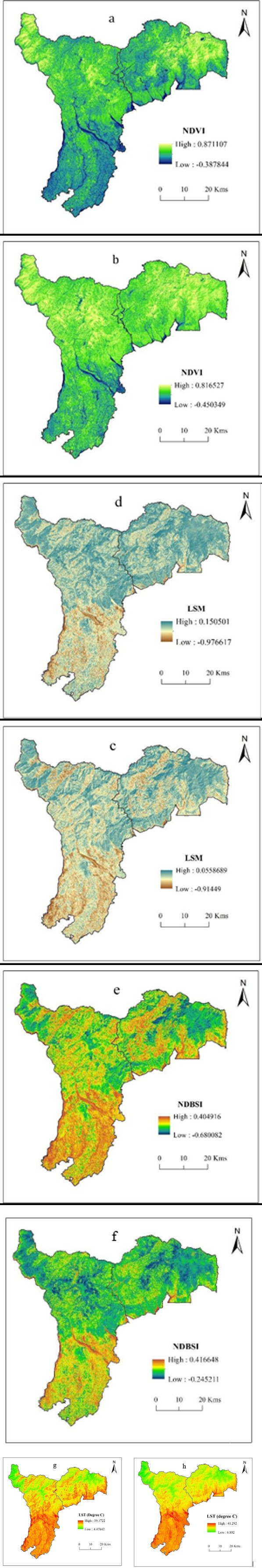
Table 4 exhibits the descriptive statistics of RSEI indicators. From the table it can be observed that NDBSI assumed as a “Pressure” indicator in our study, exhibits an increase in values increasing trend. It means values increased from -0.0898 to 0.0242 in 2022 as compared to1999. Likewise, its minimum and maximum values also increased.
This indicates increasing dryness viz. expansion of human induced built-up area and bare soil during the study period. In case of NDVI, which represents “State” of the ecosystem, the average value has increased notably from 0.3782 to 0.5135 during this period. However, its maximum and minimum values have declined, indicating partial deterioration of vegetation cover which is the result of increase in built-up areas in lower elevations, expansion of tea plantation along hill slopes, and degradation of shrublands and scrubs [28].
State Forest Report of the year 2001, 2011 and 2021 also shows an increase in both open and dense forest cover during the last two decades (State Forest Report 2001, 2011 and 2021). On the other hand, the mean value of both the “Response” indicators viz. LSM and LST have increased from -0.1071 to -0.0329 and 23.63° to 24.92° respectively from 1999 to 2022. Though LSM has increased but its negative values indicate the lack of soil moisture over the region.
LST which was in the range of 4.5-39.2°C in 1999 has shown an upward trend 6.9-41.3°C in 2022. Its minimum and maximum values have increased by 2.4°C and 2.1°C respectively.
Kumar, et al. mentioned an increase of 0.5°C to 1.5°C in mean temperature in the entire Darjeeling region in last 15 years, especially in the block in the northern, western to the southern part of Darjeeling region.
Thus, the increase of pressure index (human induced LULC change) has contributed to reduction of vegetation cover (forests) in some places, but the value of greenness is high because densely vegetated areas have converted more into croplands and tea plantation as compared to built-up and bare soil areas.
Therefore, an increase in pressure (NDBSI) and state (NDVI) index have influenced response indices (LSM and LST); which ultimately have a significant and comprehensive contribution to RSEI (Figure 3).
Assessment of Ecological Environmental Quality (EEQ)
PCA Results The RSEIs of Darjeeling district for 1999 and 2022 was computed through Principal Component Analysis of the four indicators and their contributions. Table 5 exhibits the results of PCA. PC1 with highest eigen values (78.82% in 1999) and (81.6% in 2022) contains the most variable information of the four metrics, compared with PC2, PC3, and PC4 and is represented as RSEI. PC1 has both positive and negative signs, which indicates the positive and negative roles of the indicators in the ecological environment. Here NDVI and LSM have negative signs whereas NDBSI and LST have positive signs which contradicts the reality. In the real world NDVI and LSM are assumed to be positive indicators while NDBSI and LST are assumed to be negative indicators for an ecological environment. Hence PC1 is rectified using equation 14.1.
| Year | 1999 | 2022 | ||||||
|---|---|---|---|---|---|---|---|---|
| Indicators | PC1 | PC2 | PC3 | PC4 | PC1 | PC2 | PC3 | PC4 |
| NDVI | -0.3815 | 0.74708 | 0.52599 | 0.14009 | -0.41 | 0.44842 | 0.73835 | 0.29262 |
| LSM | -0.2833 | 0.02287 | -0.4618 | 0.84025 | -0.1545 | 0.05742 | -0.4653 | 0.86965 |
| NDBSI | 0.50582 | -0.2807 | 0.62645 | 0.52242 | 0.64364 | -0.4509 | 0.47369 | 0.39758 |
| LST | 0.71995 | 0.60212 | -0.3431 | 0.03781 | 0.62748 | 0.76963 | -0.118 | -0.0025 |
| Eigenvalues | 0.01601 | 0.00252 | 0.00165 | 0.00013 | 0.01836 | 0.00343 | 0.00067 | 0.00004 |
| Percentage of eigenvalues | 78.82 | 12.42 | 8.11 | 0.64 | 81.6 | 15.23 | 2.99 | 0.17 |
| Accumulative of eigenvalues | 78.82 | 91.24 | 99.35 | 100 | 81.6 | 96.83 | 99.82 | 100 |
Table 5: Result of Principal Component Analysis (PCA) of RSEI (PC1) using four ecological indicators.
Note: PCA loads of NDVI and LSM have negative signs, causing RSEI0 (PC1) to show lower values for good ecological conditions and higher values for poor ecological conditions,
![Figure 3: Distribution of Ecological Indicators (NDVI, LSM, NDBSI & LST) NDBSI & LST) over Darjeeling and Kalimpong Districts during 1999 and 2022 [NDVI 1999 (a), NDVI 2022 (b), LSM 1999 (c), LSM 2022 (d), NDBSI 1999 (e), NDBSI 2022 (f), LST 1999 (g), LST 2022 (h)].](/fulltextimages/13778/fig_3.jpeg)
as mentioned earlier. Reverse process of subtraction of RSEI0 (PC1) from 1 will make the conversion (Equation 14.1), which will make NDVI and LSM values positive in PC1 or RSEI.
Spatio-Temporal Distribution and Change in Ecological Environmental Quality (EEQ) using RSEI
The mean RSEI value of the study area was 0.49 in 1999 and 0.58 in 2022 (Table 4) indicating an acceptable (Level 3) Ecological Environmental Quality of the study area (Table 3). Spatially higher Ecological Environmental Quality (EEQ) is observed in the north which is the part of Darjeeling Himalayas. Less human intervention owing to extremely rugged terrain and the presence of the two biosphere reserves viz. Singalila Forest in the north-west and Neora Valley National Park in the north-east has preserved the natural environment here. On the other hand, low EEQ is found in the southern part called the Terai region (Figure 4). It is acceptable to poor, and very poor in some cases. It is a plain area characterised by intense human intervention and bustling anthropogenic activities. There is very high concentration of rural and urban settlements, Siliguri the largest urban centre of the study area is located here. Besides, it has vast expanse of agricultural land, low vegetation cover and dense network of transportation which has significantly altered the natural ecosystem.
Area statistics of RSEI classes (Figure 5) shows that more than 60% area was under Level 3 (acceptable) and Level 4 (good) in 1999, which increased to 78% in 2022. Area under acceptable ecological conditions was 37.46% in 1999 which reduced to 33.3% during 2022. On the other hand, area under very good and good ecological conditions increased from 4.55% to 7.14% and 23.42% to 44.7% during 1999 and 2022 respectively. Likewise, area under poor, and very poor ecological conditions reduced from 31.49% to 13.94% and 3.08% to 0.91% respectively during the study period (Figure 5).
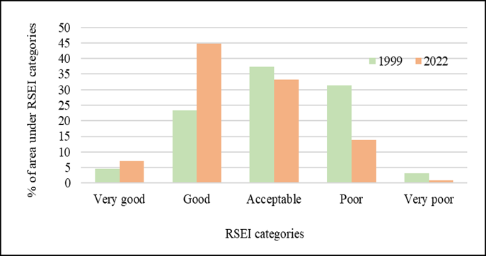
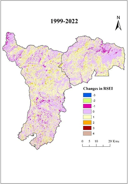
Table 6 exhibits the type of change that has occurred in the Ecological Environmental Quality (EEQ) of the study area in 2022 as compared to 1999. From the table it can be observed that 47.41% area had stable conditions with no change, there was degradation in 3.99 % area and 48.60% area had improvement in EEQ. Improvement in EEQ is observed in all parts of the study area. On the other hand, ecologically degraded areas are seen in the pockets of north- eastern, north-western and southern parts of the study area whereas ecologically stable area is concentrated in the northern part (Figure 6).
| Ecological change type | Ecological change sub-type | Changes in RSEI (1999- 2022) | Area in sq.km | Area in (%) | ||
|---|---|---|---|---|---|---|
| Area under each sub-type | Area in total | Percent of area under each sub- type | Percent of area in total | |||
| Degraded | Highly Degraded | -3 | 0.0009 | 125.586 | 0.00002861 | 3.99 |
| Moderately Degraded | -2 | 1.1826 | 0.04 | |||
| Slightly Degraded | -1 | 124.4025 | 3.95 | |||
| Stable | No Change | 0 | 1491.21 | 1491.21 | 47.41 | 47.41 |
| Improved | Slightly improved | 1 | 1411.9056 | 1528.81 | 44.88 | 48.6 |
| Moderately improved | 2 | 115.2477 | 3.66 | |||
| Highly improved | 3 | 1.6587 | 0.05 |
Table 6: Percentage of area under each ecological change type.
Relationship of RSEI with the Ecological Indicators
| 1999 | 2022 | |||||||||
|---|---|---|---|---|---|---|---|---|---|---|
| RSEI | LST | NDBSI | LSM | NDVI | RSEI | LST | NDBSI | LSM | NDVI | |
| RSEI | 1 | -0.94 | -0.91 | 0.86 | 0.71 | 1 | -0.88 | -0.95 | 0.85 | 0.85 |
| LST | -0.94 | 1 | 0.75 | -0.74 | -0.52 | -0.88 | 1 | 0.7 | -0.68 | -0.56 |
| NDBSI | -0.91 | 0.75 | 1 | -0.93 | -0.64 | -0.95 | 0.7 | 1 | -0.89 | -0.89 |
| LSM | 0.86 | -0.74 | -0.93 | 1 | 0.49 | 0.85 | -0.68 | -0.89 | 1 | 0.63 |
| NDVI | 0.71 | -0.52 | -0.64 | 0.49 | 1 | 0.85 | -0.56 | -0.89 | 0.63 | 1 |
| Mean | 0.86 | 0.74 | 0.807 | 0.76 | 0.59 | 0.88 | 0.71 | 0.857 | 0.76 | 0.73 |
Table 7: Correlation matrix of RSEI and four ecological indicators in the year 1999 and 2022.
*Mean values are calculated by averaging the other 4 values, for example, Mean RSEI for 1999 = (0.94+0.91+0.86+0.71)/4 = 0.855 Table 7: Correlation matrix of RSEI and four ecological indicators in the year 1999 and 2022.
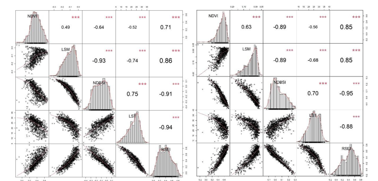
We have also assessed the relationship among RSEI and the four individual indicators in this study (Table 7 & Figure 7), RSEI is positively correlated with NDVI and LSM, while it has strong negative correlation with NDBSI and LST. The value is more than 0.80 in both the cases. Individually NDVI has positive correlation with LSM (r = 0.49 in 1999 and r = 0.63 in 2022), but is negatively correlated with NDBSI (r = -0.64 in 1999 and r = -0.89 in 2022) and LST (r = -0.52 in 1999, r = -0.56 in 2022). Likewise, LSM has high negative correlation with NDBSI. On the other hand, NDBSI has a positive correlation with LST (r = 0.75 and r = 0.70 for the 1999 and 2022 respectively), as built-up areas and bare soil are responsible for the trapping temperature and thus allowing the LST to rise.
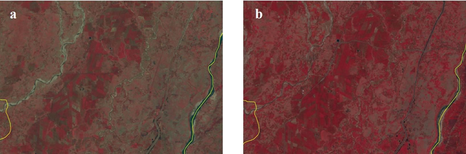
Detecting a region’s ecological status and its spatio- temporal changes poses a significant challenge due to difficulty in producing time series of ecological images showing ecological status. The RSEI technique is distinct from other approaches because its results not only produce a single numeric value but also a comprehensive ecological- status image that depicts differences in regional ecological conditions. This study on the ecological quality of Darjeeling and Kalimpong Districts reveals an improvement in the ecological quality of the study area. This is because area under forests has increased by 154 km2 in the last two decades (State Forest Report 2001, 2011, 2021). Although the built- up area has also increased but it is less than the increase in area under forests. Moreover, the contribution of vegetation to the PC1-based RSEI measurement is much higher than that of built-up land. The study also found a significant spatial difference in the ecological quality, the northern parts of the study area which are a part of the Darjeeling Himalayas have high EEQ as compared to the southern parts. This is because while the northern parts are covered with thick forest cover and biosphere reserves, the southern part, the Tarai region is bustling with anthropogenic activities. Much of the forest cover has been transformed into human settlements, plantations or agricultural fields (Figures 8 & 9). It is for this very reason that the NDVI and LSM values are higher in the northern part whereas NDBSI and LST values are high in the southern part for both 1999 and 2022 (Figure 3).
RSEI Validation
To analyze the effectiveness of the ecological index, the outcomes are verified by Location-based, Categorization-based and Correlation-based comparisons methods.
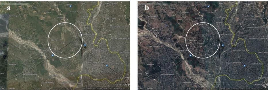
![Figure 9: Google Earth images showing built-up areas expansion and reduction of green areas, parts of Siliguri Sub-division in 1999 (a) and 2022 (b) [Image Source: Google Earth Pro].](/fulltextimages/13778/fig_9.png)
In the location-based validation, the 2022 FCC of Landsat 9 OLI was carefully examined for each level of RSEI values and the typical sample image of each RSEI level was picked (Figure 10). From the sample images it is observed that vegetation cover tended to decrease with decreasing RSEI values whereas man-made activities increased.
| RSEI Classes | 1999 | 2022 | |||||||
|---|---|---|---|---|---|---|---|---|---|
| NDBSI | NDVI | LSM | LST | NDBSI | NDVI | LSM | LST | ||
| 0-0.2 | Very Poor | 0.82 | 0.23 | 0.4 | 0.9 | 0.81 | 0.26 | 0.4 | 0.8 |
| 0.2-0.4 | Poor | 0.6 | 0.5 | 0.8 | 0.6 | 0.55 | 0.59 | 0.8 | 0.6 |
| 0.4-0.6 | Acceptable | 0.51 | 0.59 | 0.8 | 0.5 | 0.43 | 0.7 | 0.8 | 0.5 |
| 0.6-0.8 | Good | 0.43 | 0.67 | 0.9 | 0.4 | 0.32 | 0.78 | 0.8 | 0.4 |
| 0.8-1.0 | Very Good | 0.19 | 0.86 | 0.9 | 0.2 | 0.13 | 0.91 | 0.9 | 0.2 |
Table 8: Normalised mean values of each ecological indicator within the range of RSEI classes in 1999 and 2022.
In the case of categorization method, the mean of the normalised values of the four ecological indicators within different RSEI classes is considered. The very poor and poor RSEI classes have very high mean value of NDBSI and LST which represent the built-up areas and bare lands whereas, in the case of good and very good classes NDVI and LSM values dominate for both years under study (Table 8).
Likewise, the results of correlation matrix show that the mean correlation coefficients between RSEI and each variable in 1999 and 2022 (0.855 and 0.882) was higher than any other single index value (Table 7).
Also, the mean RSEI value increased in 2022 as compared to 1999 indicating an improvement in the EEQ of the study area.
Limitations and Future Scope
In the present study, multiple remote sensing indices (RSEI) are used to evaluate the ecological environment of the study region in a comprehensive way. However, use of these indices have its own drawbacks too. For instance, if remote sensing data is unavailable, it becomes difficult to extract information for that specific period. Atmospheric disturbances may interare in mainitaining the quality of data, and these datasets often fail to capture micro-ecological changes within the region.
However, in case of mountain areas, ecosystem is more fragile, with their environmental quality being highly sensitive to natural factors and human activities. Thus, to obtain a more comprehensive and scientific evaluation, studies should consider additional natural and socio-economic factors that influence the RSEI. Also, field investigation regarding the ecological status of the area can be incorporated to develop a better understanding of EEQ.
Conclusion
In the present study we have used Remote Sensing based Ecological Index (RSEI) within PSR framework to assess the change in EEQ of Darjeeling and Kalimpong Districts during 1999 and 2022 using Landsat Data. The output is relatable to the local and regional ecological conditions of the study area. As the RSEI images are produced using PCA, the study is free from subjective bias and the indicators are correlated in a single dimension.
Results indicate that from 1999 to 2022 the overall ecological conditions and environmental quality (EEQ) has improved in Darjeeling and Kalimpong Districts with sporadic degradation in some areas. The northern part of the district (Darjeeling Himalaya) is ecologically much better as compared to the southern parts of the district (Terai region) due to less human intervention. As per RSEI categories areas with very good (0.8-1.0) and good (0.6-0.8) EEQ have increased whereas areas under acceptable (0.4-0.6), poor (0.2-0.4) and very poor (0-0.2) categories have decreased, resulting in overall improvement in 2022 as compared to 1999. Based on the average RSEI values ecological environment quality of the study area has improved by 15% during 1999-2022. Reduction of poor ecological areas and enhancement of good ecological areas are responsible for the overall improvement of EEQ in the region. But in both years the mean RSEI values (0.49 in 1999 and 0.58 in 2022) are in acceptable categories (Level 3). Overall, the study offers significant insights into the eco-environment quality of Darjeeling and Kalimpong Districts over the past two decades, highlighting key areas that require intervention. The findings can guide policymakers and managers in developing and implementing strategies to protect and enhance regional ecological conditions. Continued research and monitoring are crucial to track changes and assess the long-term effectiveness of conservation efforts.
Declarations
Ethical approval: All authors have read, understood, and have complied as applicable with the statement on “Ethical responsibilities of Authors” as found in the “Instructions for Authors” and are aware that with minor exceptions, no changes can be made to authorship once the paper is submitted. Compliance with ethical standards: This article does not contain any studies with human participants or animals performed by any of the authors. Funding: No funding was received to assist with the preparation of this manuscript. Data availability: All data and materials of the research are included in this manuscript. The freely accessible data utilized for this investigation is available at: https:// earthexplorer.usgs.gov/ Competing Interest: The authors declare that they have no known competing financial interests or personal relationships that could have appeared to influence the work reported in this paper.
References
-
Ali E (2018) Spatio-Temporal Changes of land uses and land values in Mirik Municipality of Darjeeling District, West Bengal. International Journal of Scientific Research in Science and Technology 4(5): 1228-1243.
-
Baig MHA, Zhang L, Shuai T, Tong Q (2014) Derivation of a tasselled cap transformation based on Landsat 8 at-satellite reflectance. Remote Sensing Letters 5(5): 423-431.
-
Basak A (2018) Geographical study on urbanization and associated problems in North Bengal. Darjeeling.
-
Bhutia DS (2015) A Spatio-Temporal Study on Urbanization in the Darjeeling Himalaya: A Demographic Perspective. IOSR Journal Of Humanities And Social Science (IOSR-JHSS) 20(4): 10-18.
-
Bhutia S (2015) A Spatio-Temporal Study on Urbanization in the Darjeeling Himalaya: A Demographic Perspective. IOSR Journal Of Humanities And Social Science 20(4): 10-18.
-
Boori MS, Choudhary K, Paringer R, Kupriyanov A (2021a) Eco-environmental quality assessment based on pressure-state-response framework by remote sensing and GIS. Remote Sensing Applications: Society and Environment 23: 100530.
-
Boori MS, Choudhary K, Paringer R, Kupriyanov A (2021b) Spatiotemporal ecological vulnerability analysis with statistical correlation based on satellite remote sensing in Samara, Russia. Journal of Environmental Management 285: 112138.
-
Borkin D, Némethová A, Michaľčonok G, Maiorov K (2019) Impact of Data Normalization on Classification Model Accuracy. Research Papers Faculty of Materials Science and Technology Slovak University of Technology 27(45): 79-84.
-
Bose A, Chowdhury IR (2020) Monitoring and modeling of spatio-temporal urban expansion and land-use/land- cover change using markov chain model: a case study in Siliguri Metropolitan area, West Bengal, India. Modeling Earth Systems and Environment 6(4): 2235-2249.
-
Crist EP (1985) A TM Tasseled Cap equivalent transformation for reflectance factor data. Remote Sensing of Environment 17(3): 301-306.
-
Desai M (2013) Darjeeling Census Handbook, Census of India 2011, West bengal. Routledge Handbook of Indian Politics pp: 1-448.
-
Guha S, Govil H, Dey A, Gill N (2018) Analytical study of land surface temperature with NDVI and NDBI using Landsat 8 OLI and TIRS data in Florence and Naples city, Italy Subhanil Guha, Himanshu Govil, Anindita Dey & Neetu Gill. European Journal of Remote Sensing 51(1): 667-678.
-
Halder S, Bose S (2024a) Comparative study on remote sensing-based indices for urban ecology assessment: A case study of 12 urban centers in the metropolitan area of eastern India. Journal of Earth System Science 133(2).
-
Halder S, Bose S (2024b) Ecological quality assessment of five smart cities in India: a remote sensing index- based analysis. International Journal of Environmental Science and Technology 21(4): 4101-4118.
-
Hu X, Xu H (2019) A new remote sensing index based on the pressure-state-response framework to assess regional ecological change. Environmental Science and Pollution Research 26(6): 5381-5393.
-
Jiang F, Zhang Y, Li J, Sun Z (2021) Research on remote sensing ecological environmental assessment method optimized by regional scale. Environmental Science and Pollution Research pp: 68174-68187.
-
Maity S, Das S, Pattanayak JM, Bera B, Shit PK (2022) Assessment of ecological environment quality in Kolkata urban agglomeration, India. Urban Ecosystems 25(4): 1137-1154.
-
Mell IC, Sturzaker J (2014) Sustainable urban development in tightly constrained areas: A case study of Darjeeling, India. International Journal of Urban Sustainable Development 6(1): 65-88.
-
Mor S (2013) Critical Ecosystem Modeling and Analysis of Darjeeling District, West Bengal, India Using Geospatial Techniques.
-
Ojha K (1890) 19th Century Darjeelinc O Tudy In Urbanization.
-
Pettorelli N, Vik JO, Mysterud A, Gaillard JM, Tucker CJ, et al. (2005) Using the satellite-derived NDVI to assess ecological responses to environmental change. Trends in Ecology and Evolution 20(9): 503-510.
-
Philip A (2024) Dynamic monitoring and analysis of ecological quality based on RSEI: a case study of Akkulam-Veli Lake basin of Thiruvananthapuram city, Kerala, India. Geology, Ecology, and Landscapes.
-
Sharma RP (2012) A Study in environmental degradation in the Darjeeling hill areas. Darjeeling.
-
Sobrino JA, Jiménez-Muñoz JC, Paolini L (2004) Land surface temperature retrieval from LANDSAT TM 5. Remote Sensing of Environment 90(4): 434-440.
-
Xia QQ, Chen YN, Zhang XQ, Ding JL (2022) Spatiotemporal Changes in Ecological Quality and Its Associated Driving Factors in Central Asia. Remote Sensing 14(14): 1-16.
-
Xu H, Wang M, Shi T, Guan H, Fang C, et al. (2018) Prediction of ecological effects of potential population and impervious surface increases using a remote sensing based ecological index (RSEI). Ecological Indicators 93: 730-740.
-
Xu H, Wang Y, Guan H, Shi T, Hu X (2019) Detecting ecological changes with a remote sensing based ecological index (RSEI) produced time series and change vector analysis. Remote Sensing 11(20): 1-24.
-
Yue H, Liu Y, Li Y, Lu Y (2019) Eco-environmental quality assessment in china’s 35 major cities based on remote sensing ecological index. IEEE Access 7: 51295-51311.
-
Zewdie W, Csaplovics E, Inostroza L (2017) Monitoring ecosystem dynamics in northwestern Ethiopia using NDVI and climate variables to assess long term trends in dryland vegetation variability. Applied Geography 79: 167-178.
- Community Forestry Enterprises as a Model for Sustainable Forest Development: The Case Of The "Baja Tarahumara" in Chihuahua, Mexico
- Ecological and Socio-Economic Impacts of Chromolaena odorata and Mesosphaerum suaveolens, Two Invasive Alien Species in Central and Southern Benin, West Africa
- Epigenetic Sustainability: Modeling the Human Factor as a Natural Resource through Science 4.0 and the NR3C1 Biological Pilot
- Growth-at-Risk: A Framework for Assessing Economic Vulnerability
- The Rural Territory as a Socioecological System for the Management of Public Policy for Sustainable Rural Development
- Transition Risks in a Small Open Economy: An EDSGE Model with Blue Firms, Financial Frictions and Macroprudential Policy